Aerosol Size Distribution
Overview
This module implements the multi-modal lognormal aerosol size distribution parameterization described in Chapter 8 ("Properties of the Atmospheric Aerosol") of Seinfeld and Pandis (2006).
The aerosol particle size distribution is represented as a sum of lognormal modes (Eq. 8.54), where each mode is characterized by a number concentration $N_i$, geometric median diameter $D_{g,i}$, and geometric standard deviation $\sigma_{g,i}$. This parameterization is widely used to represent the number, surface area, and volume distributions of atmospheric aerosol populations across different environments.
Reference: Seinfeld, J.H. and Pandis, S.N. (2006). Atmospheric Chemistry and Physics: From Air Pollution to Climate Change, 2nd Edition, John Wiley & Sons, Chapter 8, pp. 350–395.
Aerosol.AerosolDistribution — Function
AerosolDistribution(n_modes=3; name=:AerosolDistribution)Multi-modal lognormal aerosol size distribution following the parameterization of Seinfeld and Pandis (2006), Chapter 8, "Properties of the Atmospheric Aerosol", in Atmospheric Chemistry and Physics: From Air Pollution to Climate Change, 2nd Edition, John Wiley & Sons.
The model represents the aerosol number, surface area, and volume distributions as a sum of n_modes lognormal modes (Eq. 8.54). Each mode i is characterized by three parameters:
N[i]: total number concentration of modeiD_g[i]: geometric median diameter of modeilogσ[i]: log10 of the geometric standard deviation of modei
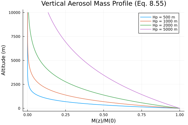
The implementation also includes the vertical mass profile (Eq. 8.55).
Default parameter values correspond to the "Urban" distribution from Table 8.3.
Aerosol.UrbanAerosol — Function
UrbanAerosol(; name=:UrbanAerosol)Urban aerosol size distribution from Table 8.3 of Seinfeld and Pandis (2006).
Three lognormal modes with parameters:
- Mode 1: nucleation mode (N=9.93×10⁴ cm⁻³, Dg=0.013 μm, log σ=0.245)
- Mode 2: Aitken mode (N=1.11×10³ cm⁻³, Dg=0.014 μm, log σ=0.666)
- Mode 3: accumulation mode (N=3.64×10⁴ cm⁻³, Dg=0.050 μm, log σ=0.337)
Aerosol.MarineAerosol — Function
MarineAerosol(; name=:MarineAerosol)Marine aerosol size distribution from Table 8.3 of Seinfeld and Pandis (2006).
Three lognormal modes with parameters:
- Mode 1: (N=133 cm⁻³, Dg=0.008 μm, log σ=0.657)
- Mode 2: (N=66.6 cm⁻³, Dg=0.266 μm, log σ=0.210)
- Mode 3: (N=3.1 cm⁻³, Dg=0.58 μm, log σ=0.396)
Aerosol.RuralAerosol — Function
RuralAerosol(; name=:RuralAerosol)Rural aerosol size distribution from Table 8.3 of Seinfeld and Pandis (2006).
Three lognormal modes with parameters:
- Mode 1: (N=6.65×10³ cm⁻³, Dg=0.015 μm, log σ=0.225)
- Mode 2: (N=147 cm⁻³, Dg=0.054 μm, log σ=0.557)
- Mode 3: (N=1990 cm⁻³, Dg=0.084 μm, log σ=0.266)
Aerosol.RemoteContinentalAerosol — Function
RemoteContinentalAerosol(; name=:RemoteContinentalAerosol)Remote continental aerosol size distribution from Table 8.3 of Seinfeld and Pandis (2006).
Three lognormal modes with parameters:
- Mode 1: (N=3200 cm⁻³, Dg=0.020 μm, log σ=0.161)
- Mode 2: (N=2900 cm⁻³, Dg=0.116 μm, log σ=0.217)
- Mode 3: (N=0.300 cm⁻³, Dg=1.800 μm, log σ=0.380)
Aerosol.FreeTroposphereAerosol — Function
FreeTroposphereAerosol(; name=:FreeTroposphereAerosol)Free troposphere aerosol size distribution from Table 8.3 of Seinfeld and Pandis (2006).
Three lognormal modes with parameters:
- Mode 1: (N=129 cm⁻³, Dg=0.007 μm, log σ=0.645)
- Mode 2: (N=59.7 cm⁻³, Dg=0.250 μm, log σ=0.253)
- Mode 3: (N=63.5 cm⁻³, Dg=0.520 μm, log σ=0.425)
Aerosol.PolarAerosol — Function
PolarAerosol(; name=:PolarAerosol)Polar aerosol size distribution from Table 8.3 of Seinfeld and Pandis (2006).
Three lognormal modes with parameters:
- Mode 1: (N=21.7 cm⁻³, Dg=0.138 μm, log σ=0.245)
- Mode 2: (N=0.186 cm⁻³, Dg=0.75 μm, log σ=0.300)
- Mode 3: (N=3×10⁻⁴ cm⁻³, Dg=8.6 μm, log σ=0.291)
Aerosol.DesertAerosol — Function
DesertAerosol(; name=:DesertAerosol)Desert aerosol size distribution from Table 8.3 of Seinfeld and Pandis (2006).
Three lognormal modes with parameters:
- Mode 1: (N=726 cm⁻³, Dg=0.002 μm, log σ=0.247)
- Mode 2: (N=114 cm⁻³, Dg=0.038 μm, log σ=0.770)
- Mode 3: (N=0.178 cm⁻³, Dg=21.60 μm, log σ=0.438)
Implementation
The AerosolDistribution component represents a multi-modal lognormal distribution with the following key equations:
- Number distribution (Eq. 8.54): $\frac{dN}{d\log D_p} = \sum_i \frac{N_i}{\sqrt{2\pi}\,\log\sigma_{g,i}} \exp\!\left(-\frac{(\log D_p - \log D_{g,i})^2}{2\log^2\sigma_{g,i}}\right)$
- Surface area distribution (Eq. 8.49/8.50): Same form with surface area median diameter $D_{s,i} = D_{g,i}\exp(2\ln^2\sigma_{g,i})$
- Volume distribution (Eq. 8.52/8.53): Same form with volume median diameter $D_{v,i} = D_{g,i}\exp(3\ln^2\sigma_{g,i})$
- Vertical mass profile (Eq. 8.55): $M(z) = M(0)\exp(-z/H_p)$
Seven predefined aerosol distribution types are provided from Table 8.3, each with three lognormal modes calibrated to represent typical atmospheric conditions.
State Variables
using DataFrames, ModelingToolkit, Symbolics, Aerosol, DynamicQuantities

sys = AerosolDistribution(3)
vars = unknowns(sys)
DataFrame(
    :Name => [string(Symbolics.tosymbol(v, escape = false)) for v in vars],
    :Units => [dimension(ModelingToolkit.get_unit(v)) for v in vars],
    :Description => [ModelingToolkit.getdescription(v) for v in vars]
)| Row | Name | Units | Description |
|---|---|---|---|
| String | Dimensio… | String | |
| 1 | n_N_o | m⁻³ | Number distribution dN/d(log D_p) |
| 2 | n_S_o | m⁻¹ | Surface area distribution dS/d(log D_p) |
| 3 | n_V_o | Volume distribution dV/d(log D_p) | |
| 4 | N_t | m⁻³ | Total number concentration |
| 5 | S_t | m⁻¹ | Total surface area concentration |
| 6 | V_t | Total volume concentration | |
| 7 | D_s | m | Surface area median diameter |
| 8 | D_v | m | Volume median diameter |
| 9 | D_bar | m | Mean diameter |
| 10 | M_z | Mass concentration vertical profile ratio M(z)/M(0) (dimensionless) |
Parameters
pars = parameters(sys)
DataFrame(
    :Name => [string(Symbolics.tosymbol(p, escape = false)) for p in pars],
    :Units => [dimension(ModelingToolkit.get_unit(p)) for p in pars],
    :Description => [ModelingToolkit.getdescription(p) for p in pars]
)| Row | Name | Units | Description |
|---|---|---|---|
| String | Dimensio… | String | |
| 1 | D_p | m | Particle diameter evaluation point |
| 2 | D_g | m | Geometric median diameter of mode i |
| 3 | logσ | Log10 of geometric standard deviation of mode i (dimensionless) | |
| 4 | N | m⁻³ | Number concentration of mode i |
| 5 | π_c | Pi | |
| 6 | ln10 | Natural log of 10 | |
| 7 | z | m | Altitude above surface |
| 8 | H_p | m | Aerosol mass scale height |
Equations
eqs = equations(sys)10-element Vector{Symbolics.Equation}:
n_N_o(t) ~ (N[1]*exp((-(log10(D_p / D_g[1])^2)) / (2(logσ[1]^2)))) / (logσ[1]*sqrt(2π_c)) + (N[2]*exp((-(log10(D_p / D_g[2])^2)) / (2(logσ[2]^2)))) / (logσ[2]*sqrt(2π_c)) + (N[3]*exp((-(log10(D_p / D_g[3])^2)) / (2(logσ[3]^2)))) / (logσ[3]*sqrt(2π_c))
n_S_o(t) ~ ((D_g[1]^2)*N[1]*exp((-(log10(D_p / (D_g[1]*exp(2(ln10^2)*(logσ[1]^2))))^2)) / (2(logσ[1]^2)))*(exp(2(ln10^2)*(logσ[1]^2))^2)*π_c) / (logσ[1]*sqrt(2π_c)) + ((D_g[2]^2)*N[2]*exp((-(log10(D_p / (D_g[2]*exp(2(ln10^2)*(logσ[2]^2))))^2)) / (2(logσ[2]^2)))*(exp(2(ln10^2)*(logσ[2]^2))^2)*π_c) / (logσ[2]*sqrt(2π_c)) + ((D_g[3]^2)*N[3]*exp((-(log10(D_p / (D_g[3]*exp(2(ln10^2)*(logσ[3]^2))))^2)) / (2(logσ[3]^2)))*(exp(2(ln10^2)*(logσ[3]^2))^2)*π_c) / (logσ[3]*sqrt(2π_c))
n_V_o(t) ~ ((D_g[1]^3)*N[1]*exp((-(log10(D_p / (D_g[1]*exp(3(ln10^2)*(logσ[1]^2))))^2)) / (2(logσ[1]^2)))*(exp(3(ln10^2)*(logσ[1]^2))^3)*π_c) / (6logσ[1]*sqrt(2π_c)) + ((D_g[2]^3)*N[2]*exp((-(log10(D_p / (D_g[2]*exp(3(ln10^2)*(logσ[2]^2))))^2)) / (2(logσ[2]^2)))*(exp(3(ln10^2)*(logσ[2]^2))^3)*π_c) / (6logσ[2]*sqrt(2π_c)) + ((D_g[3]^3)*N[3]*exp((-(log10(D_p / (D_g[3]*exp(3(ln10^2)*(logσ[3]^2))))^2)) / (2(logσ[3]^2)))*(exp(3(ln10^2)*(logσ[3]^2))^3)*π_c) / (6logσ[3]*sqrt(2π_c))
N_t(t) ~ N[1] + N[2] + N[3]
S_t(t) ~ (D_g[1]^2)*N[1]*exp(2(ln10^2)*(logσ[1]^2))*π_c + (D_g[2]^2)*N[2]*exp(2(ln10^2)*(logσ[2]^2))*π_c + (D_g[3]^2)*N[3]*exp(2(ln10^2)*(logσ[3]^2))*π_c
V_t(t) ~ (1//6)*(D_g[1]^3)*N[1]*exp(4.5(ln10^2)*(logσ[1]^2))*π_c + (1//6)*(D_g[2]^3)*N[2]*exp(4.5(ln10^2)*(logσ[2]^2))*π_c + (1//6)*(D_g[3]^3)*N[3]*exp(4.5(ln10^2)*(logσ[3]^2))*π_c
D_s(t) ~ D_g[1]*exp(2(ln10^2)*(logσ[1]^2))
D_v(t) ~ D_g[1]*exp(3(ln10^2)*(logσ[1]^2))
D_bar(t) ~ D_g[1]*exp(0.5(ln10^2)*(logσ[1]^2))
M_z(t) ~ exp((-z) / H_p)Table 8.3: Model Aerosol Distributions
The following table reproduces Table 8.3 from Seinfeld and Pandis (2006), showing the parameters for seven model aerosol distributions expressed as the sum of three lognormal modes. Units: N in cm⁻³, D_p in μm.
using DataFrames

# Table 8.3 data (in original units from the book)
table_data = [
    ("Urban", 9.93e4, 0.013, 0.245, 1.11e3, 0.014, 0.666, 3.64e4, 0.050, 0.337),
    ("Marine", 133, 0.008, 0.657, 66.6, 0.266, 0.210, 3.1, 0.58, 0.396),
    ("Rural", 6650, 0.015, 0.225, 147, 0.054, 0.557, 1990, 0.084, 0.266),
    ("Remote continental", 3200, 0.020, 0.161, 2900, 0.116, 0.217, 0.3, 1.8, 0.380),
    ("Free troposphere", 129, 0.007, 0.645, 59.7, 0.250, 0.253, 63.5, 0.52, 0.425),
    ("Polar", 21.7, 0.138, 0.245, 0.186, 0.75, 0.300, 3e-4, 8.6, 0.291),
    ("Desert", 726, 0.002, 0.247, 114, 0.038, 0.770, 0.178, 21.6, 0.438)
]

DataFrame(
    :Type => [d[1] for d in table_data],
    Symbol("N₁ (cm⁻³)") => [d[2] for d in table_data],
    Symbol("Dₚ₁ (μm)") => [d[3] for d in table_data],
    Symbol("log σ₁") => [d[4] for d in table_data],
    Symbol("N₂ (cm⁻³)") => [d[5] for d in table_data],
    Symbol("Dₚ₂ (μm)") => [d[6] for d in table_data],
    Symbol("log σ₂") => [d[7] for d in table_data],
    Symbol("N₃ (cm⁻³)") => [d[8] for d in table_data],
    Symbol("Dₚ₃ (μm)") => [d[9] for d in table_data],
    Symbol("log σ₃") => [d[10] for d in table_data]
)| Row | Type | N₁ (cm⁻³) | Dₚ₁ (μm) | log σ₁ | N₂ (cm⁻³) | Dₚ₂ (μm) | log σ₂ | N₃ (cm⁻³) | Dₚ₃ (μm) | log σ₃ |
|---|---|---|---|---|---|---|---|---|---|---|
| String | Real | Float64 | Float64 | Real | Float64 | Float64 | Real | Float64 | Float64 | |
| 1 | Urban | 99300.0 | 0.013 | 0.245 | 1110.0 | 0.014 | 0.666 | 36400.0 | 0.05 | 0.337 |
| 2 | Marine | 133 | 0.008 | 0.657 | 66.6 | 0.266 | 0.21 | 3.1 | 0.58 | 0.396 |
| 3 | Rural | 6650 | 0.015 | 0.225 | 147 | 0.054 | 0.557 | 1990 | 0.084 | 0.266 |
| 4 | Remote continental | 3200 | 0.02 | 0.161 | 2900 | 0.116 | 0.217 | 0.3 | 1.8 | 0.38 |
| 5 | Free troposphere | 129 | 0.007 | 0.645 | 59.7 | 0.25 | 0.253 | 63.5 | 0.52 | 0.425 |
| 6 | Polar | 21.7 | 0.138 | 0.245 | 0.186 | 0.75 | 0.3 | 0.0003 | 8.6 | 0.291 |
| 7 | Desert | 726 | 0.002 | 0.247 | 114 | 0.038 | 0.77 | 0.178 | 21.6 | 0.438 |
Analysis
# Helper to get the base name of a symbolic variable (part after last ₊),
# and strip the (t) suffix if present.
function get_base_name(sym)
    name = string(Symbolics.tosymbol(sym, escape = false))
    name = contains(name, "₊") ? split(name, "₊")[end] : name
    name = replace(name, r"\(t\)$" => "")
    return name
end

# Helper to evaluate a system equation's RHS by substituting parameter values.
# Handles namespaced variables by matching the actual symbols in the equation RHS.
function eval_eq(sys, var, param_vals)
    var_base = get_base_name(var)

    # Find the equation for this variable
    matching_eqs = filter(equations(sys)) do eq
        lhs_base = get_base_name(eq.lhs)
        return lhs_base == var_base
    end
    eq = only(matching_eqs)

    # Get all variables that appear in the RHS
    rhs_vars = Symbolics.get_variables(eq.rhs)

    # Build substitution dict from defaults and user-provided values
    subs = Dict{Any, Any}()

    # Collect defaults from parameters (includes constants in MTK v11)
    # Expand array parameters into indexed entries (e.g., D_g => [a,b,c] becomes D_g[1]=>a, D_g[2]=>b, D_g[3]=>c)
    defs = Dict{String, Any}()
    for s in parameters(sys)
        if ModelingToolkit.hasdefault(s)
            v = ModelingToolkit.getdefault(s)
            v = v isa Irrational ? Float64(v) : v
            k_str = string(s)
            if v isa AbstractVector
                for (i, vi) in enumerate(v)
                    defs["$(k_str)[$i]"] = vi
                end
            else
                defs[k_str] = v
            end
        end
    end

    for rv in rhs_vars
        rv_str = string(rv)

        # Check system defaults
        for (k_str, v) in defs
            if rv_str == k_str || endswith(k_str, "₊" * rv_str)
                subs[rv] = v
            end
        end

        # Check user-provided values (these override defaults)
        for (k, v) in param_vals
            k_str = string(k)
            if rv_str == k_str || endswith(k_str, "₊" * rv_str)
                subs[rv] = v
            end
        end
    end

    result = Symbolics.substitute(eq.rhs, subs)
    return Float64(eval(Symbolics.toexpr(result)))
end
Urban Aerosol Distribution (Figure 8.14)
The urban aerosol distribution from Table 8.3 shows three distinct modes: a nucleation mode, an Aitken mode, and an accumulation mode.
using Plots

urban = UrbanAerosol()

# Evaluate the system's n_N_o equation over a range of diameters
D_p_range = 10 .^ range(log10(1e-9), log10(100e-6), length = 500)
n_N_total = map(D_p_range) do D_p_val
    eval_eq(urban, urban.n_N_o, Dict(urban.D_p => D_p_val))
end

# Also evaluate individual mode contributions using single-mode systems
mode_contributions = [zeros(length(D_p_range)) for _ in 1:3]
# Get default values for the urban distribution parameters
urban_N = ModelingToolkit.getdefault(urban.N)
urban_D_g = ModelingToolkit.getdefault(urban.D_g)
urban_logσ = ModelingToolkit.getdefault(urban.logσ)
for i in 1:3
    mode_sys = AerosolDistribution(1; name = Symbol("mode_$i"))
    for (j, D_p_val) in enumerate(D_p_range)
        mode_contributions[i][j] = eval_eq(mode_sys,
            mode_sys.n_N_o,
            Dict(
                mode_sys.N[1] => urban_N[i],
                mode_sys.D_g[1] => urban_D_g[i],
                mode_sys.logσ[1] => urban_logσ[i],
                mode_sys.D_p => D_p_val
            ))
    end
end

# Convert to cm^-3 for plotting (standard convention)
p = plot(D_p_range * 1e6, n_N_total / 1e6,
    xscale = :log10, xlabel = "Particle Diameter (μm)",
    ylabel = "dN/d(log Dp) (cm⁻³)",
    label = "Total", linewidth = 2, color = :black,
    title = "Urban Aerosol Size Distribution (Table 8.3)")
for i in 1:3
    plot!(p, D_p_range * 1e6, mode_contributions[i] / 1e6,
        label = "Mode $i", linestyle = :dash)
end
p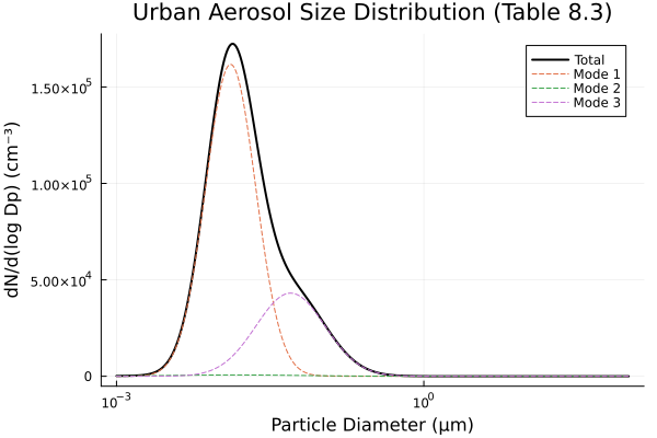
Comparison of All Aerosol Types (Figures 8.14–8.20)
The following figure compares the number distributions for all seven aerosol environment types from Table 8.3.
dist_constructors = [
    ("Desert", DesertAerosol),
    ("Free troposphere", FreeTroposphereAerosol),
    ("Marine", MarineAerosol),
    ("Polar", PolarAerosol),
    ("Remote continental", RemoteContinentalAerosol),
    ("Rural", RuralAerosol),
    ("Urban", UrbanAerosol)
]

D_p_range = 10 .^ range(log10(1e-9), log10(100e-6), length = 500)
p = plot(xlabel = "Particle Diameter (μm)", ylabel = "dN/d(log Dp) (cm⁻³)",
    xscale = :log10, yscale = :log10, legend = :topright,
    title = "Model Aerosol Size Distributions (Table 8.3)",
    ylims = (1e-3, 1e6))

for (env_name, constructor) in dist_constructors
    dist_sys = constructor()
    n_N = map(D_p_range) do D_p_val
        eval_eq(dist_sys, dist_sys.n_N_o, Dict(dist_sys.D_p => D_p_val))
    end
    # Convert from m^-3 to cm^-3 for plotting
    plot!(p, D_p_range * 1e6, n_N / 1e6, label = env_name, linewidth = 1.5)
end
p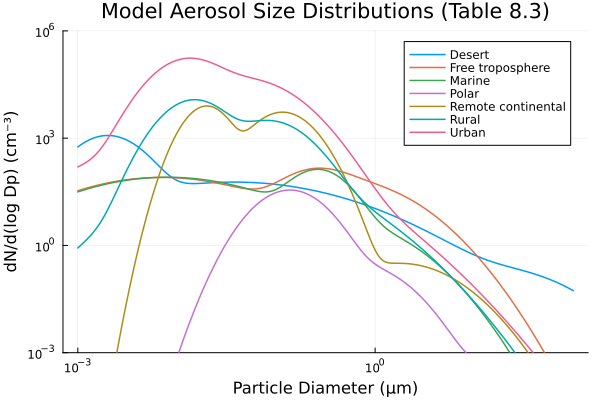
Volume Distributions
The volume distribution emphasizes larger particles and is important for understanding aerosol mass loading. For each mode, the volume distribution peaks at the volume median diameter $D_{v,i} = D_{g,i}\exp(3\ln^2\sigma_{g,i})$ (Eq. 8.53).
# Urban volume distribution using the system's n_V_o equation
urban = UrbanAerosol()
D_p_range = 10 .^ range(log10(1e-9), log10(100e-6), length = 500)

n_V_total = map(D_p_range) do D_p_val
    eval_eq(urban, urban.n_V_o, Dict(urban.D_p => D_p_val))
end

p = plot(xlabel = "Particle Diameter (μm)", ylabel = "dV/d(log Dp) (μm³/cm³)",
    xscale = :log10, title = "Urban Aerosol Volume Distribution",
    legend = :topright)

# Convert from m³/m³ to μm³/cm³: m³→μm³ is ×1e18, m⁻³→cm⁻³ is ÷1e6, net ×1e12
plot!(p, D_p_range * 1e6, n_V_total * 1e12, label = "Total", linewidth = 2, color = :black)
p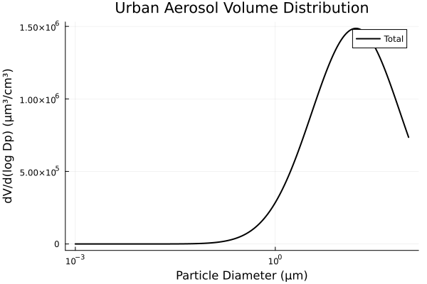
Vertical Mass Profile (Eq. 8.55)
The vertical variation of aerosol mass concentration follows an exponential decay with a characteristic scale height $H_p$.
# Evaluate the system's M_z equation for different scale heights
sys = AerosolDistribution(3)
z_range = range(0, 10000, length = 100)
H_p_values = [500, 1000, 2000, 5000]

base_params = Dict(
    sys.N[1] => 1e11, sys.D_g[1] => 1e-7, sys.logσ[1] => 0.3,
    sys.N[2] => 1e10, sys.D_g[2] => 1e-6, sys.logσ[2] => 0.3,
    sys.N[3] => 1e9, sys.D_g[3] => 1e-5, sys.logσ[3] => 0.3,
    sys.D_p => 1e-7
)

p = plot(xlabel = "M(z)/M(0)", ylabel = "Altitude (m)",
    title = "Vertical Aerosol Mass Profile (Eq. 8.55)",
    legend = :topright)

for H_p in H_p_values
    M_ratio = map(z_range) do z_val
        eval_eq(sys, sys.M_z, merge(base_params, Dict(sys.z => z_val, sys.H_p => Float64(H_p))))
    end
    plot!(p, M_ratio, z_range, label = "Hp = $H_p m", linewidth = 1.5)
end
p