Aerosol Radiative Forcing
Overview
This module implements the aerosol radiative forcing equations from Chapter 24 ("Aerosols and Climate") of Seinfeld & Pandis's "Atmospheric Chemistry and Physics" textbook. The equations describe both direct and indirect effects of aerosols on Earth's radiation budget.
Direct effects occur when aerosols scatter and absorb incoming solar radiation, modifying the planetary albedo. Indirect effects arise from aerosols acting as cloud condensation nuclei (CCN), increasing cloud droplet number concentration (CDNC) and thereby altering cloud optical properties.
Reference: Seinfeld, J. H., and Pandis, S. N. (2006). Atmospheric Chemistry and Physics: From Air Pollution to Climate Change, 2nd Edition, Chapter 24, pp. 1054-1091.
Aerosol.AerosolLayerRadiativeForcing — Function
AerosolLayerRadiativeForcing(; name=:AerosolLayerRadiativeForcing)Aerosol layer radiative forcing model from Seinfeld & Pandis (2006) Chapter 24.
This component calculates the change in outgoing radiative flux due to an aerosol layer using the scattering-absorbing model from Section 24.1. It computes the reflection and transmission coefficients, the total reflectance of the aerosol-surface system, and the change in planetary albedo.
Reference: Seinfeld, J. H., and Pandis, S. N. (2006). Atmospheric Chemistry and Physics: From Air Pollution to Climate Change, 2nd Edition, Chapter 24, Equations 24.1-24.10.
Parameters
F_0: Incident solar flux (W m⁻²)τ: Aerosol optical depth (dimensionless)ω: Single-scattering albedo (dimensionless)β: Upscatter fraction (dimensionless)R_s: Surface albedo (dimensionless)A_c: Cloud fraction (dimensionless)T_a: Atmospheric transmittance (dimensionless)
Variables (computed)
r_aer: Fraction of light reflected upward by aerosol (dimensionless)t_aer: Fraction of light transmitted through aerosol (dimensionless)R_as: Total reflectance of aerosol-surface system (dimensionless)ΔR_p: Change in planetary albedo (dimensionless)ΔF: Change in outgoing radiative flux (W m⁻²)
Aerosol.CriticalSingleScatteringAlbedo — Function
CriticalSingleScatteringAlbedo(; name=:CriticalSingleScatteringAlbedo)Component to calculate the critical single-scattering albedo (ω_crit) at which an aerosol layer transitions from cooling to heating the climate system.
From Seinfeld & Pandis (2006) Chapter 24, Equation 24.15: ωcrit = 2*Rs / (2R_s + β(1-R_s)²)
When ω > ωcrit, the aerosol causes net cooling (increased reflection). When ω < ωcrit, the aerosol causes net heating (absorption dominates).
Reference: Seinfeld, J. H., and Pandis, S. N. (2006). Atmospheric Chemistry and Physics, Chapter 24, Section 24.2.
Parameters
R_s: Surface albedo (dimensionless)β: Upscatter fraction (dimensionless)
Variables (computed)
ω_crit: Critical single-scattering albedo (dimensionless)
Aerosol.CloudOpticalDepth — Function
CloudOpticalDepth(; name=:CloudOpticalDepth)Component to calculate cloud optical depth from liquid water content and droplet number concentration.
From Seinfeld & Pandis (2006) Chapter 24, Section 24.8.1: τc = h * (9πL²N / 2ρw²)^(1/3) (Eq. 24.36)
This relates cloud optical depth to cloud thickness (h), liquid water content (L), and cloud droplet number concentration (N).
Reference: Seinfeld, J. H., and Pandis, S. N. (2006). Atmospheric Chemistry and Physics, Chapter 24, Section 24.8.1, Equations 24.34-24.36.
Parameters
h: Cloud thickness (m)L: Liquid water content (kg m⁻³)N: Cloud droplet number concentration (m⁻³)
Constants
ρ_w: Density of water (kg m⁻³)
Variables (computed)
τ_c: Cloud optical depth (dimensionless)
Aerosol.CloudAlbedo — Function
CloudAlbedo(; name=:CloudAlbedo)Component to calculate cloud albedo from optical depth using the two-stream approximation.
From Seinfeld & Pandis (2006) Chapter 24, Section 24.8.1: Rc = τc / (τ_c + γ) (Eq. 24.38, simplified form for g = 0.85)
where γ = 7.7 for an asymmetry factor g = 0.85 (typical for cloud droplets).
The general two-stream approximation (Eq. 24.37) is: Rc = √3(1-g)τc / (2 + √3(1-g)τ_c)
Reference: Seinfeld, J. H., and Pandis, S. N. (2006). Atmospheric Chemistry and Physics, Chapter 24, Section 24.8.1, Equations 24.37-24.38.
Parameters
τ_c: Cloud optical depth (dimensionless)g: Asymmetry factor (dimensionless, default 0.85)
Variables (computed)
R_c: Cloud albedo (dimensionless)γ: Denominator coefficient for two-stream approximation (dimensionless)
Aerosol.CloudAlbedoSensitivity — Function
CloudAlbedoSensitivity(; name=:CloudAlbedoSensitivity)Component to calculate the sensitivity of cloud albedo to cloud droplet number concentration (Twomey susceptibility).
From Seinfeld & Pandis (2006) Chapter 24, Section 24.8.2: dRc/dN = Rc(1-Rc)/(3N) (Eq. 24.40) dRc/d(ln N) = R_c(1-R_c)/3 (Eq. 24.41, Twomey susceptibility)
The maximum susceptibility occurs at R_c = 0.5.
Reference: Seinfeld, J. H., and Pandis, S. N. (2006). Atmospheric Chemistry and Physics, Chapter 24, Section 24.8.2, Equations 24.39-24.42.
Parameters
R_c: Cloud albedo (dimensionless)N: Cloud droplet number concentration (m⁻³)
Variables (computed)
dRc_dN: Sensitivity of cloud albedo to CDNC (m³)S: Twomey susceptibility dR_c/d(ln N) (dimensionless)
Aerosol.IndirectAerosolForcing — Function
IndirectAerosolForcing(; name=:IndirectAerosolForcing)Component to calculate the indirect radiative forcing from aerosol effects on cloud albedo (first indirect effect, or Twomey effect).
From Seinfeld & Pandis (2006) Chapter 24, Section 24.8.2: ΔFc = -F0 * Ac * Ta² * ΔRc (Eq. 24.43) ΔRc = Rc*(1-Rc)/3 * Δln(N) (Eq. 24.42)
This gives the change in shortwave forcing due to changes in cloud albedo caused by changes in cloud droplet number concentration.
Reference: Seinfeld, J. H., and Pandis, S. N. (2006). Atmospheric Chemistry and Physics, Chapter 24, Section 24.8.2, Equations 24.42-24.43.
Parameters
F_0: Incident solar flux (W m⁻²)A_c: Cloud fraction (dimensionless)T_a: Atmospheric transmittance (dimensionless)R_c: Cloud albedo (dimensionless)Δln_N: Fractional change in CDNC, Δln(N) = ΔN/N (dimensionless)
Variables (computed)
ΔR_c: Change in cloud albedo (dimensionless)ΔF_c: Change in shortwave forcing (W m⁻²)
Implementation
The module provides six @component functions that implement the key equations from Chapter 24:
- AerosolLayerRadiativeForcing: Calculates the change in outgoing radiative flux due to an aerosol layer (Eqs. 24.1-24.10)
- CriticalSingleScatteringAlbedo: Determines the boundary between aerosol cooling and heating (Eq. 24.15)
- CloudOpticalDepth: Relates cloud optical depth to microphysical properties (Eq. 24.36)
- CloudAlbedo: Computes cloud albedo from optical depth using two-stream approximation (Eqs. 24.37-24.38)
- CloudAlbedoSensitivity: Quantifies the Twomey susceptibility (Eqs. 24.40-24.41)
- IndirectAerosolForcing: Calculates the first indirect effect of aerosols on climate (Eqs. 24.42-24.43)
System Variables
using DataFrames, ModelingToolkit, Symbolics, DynamicQuantities
using Aerosol

sys = AerosolLayerRadiativeForcing()

vars = unknowns(sys)
DataFrame(
    :Name => [string(Symbolics.tosymbol(v, escape = false)) for v in vars],
    :Units => [repr(ModelingToolkit.get_unit(v)) for v in vars],
    :Description => [ModelingToolkit.getdescription(v) for v in vars]
)| Row | Name | Units | Description |
|---|---|---|---|
| String | String | String | |
| 1 | r_aer | 1.0 | Fraction of light reflected upward by aerosol |
| 2 | t_aer | 1.0 | Fraction of light transmitted through aerosol |
| 3 | R_as | 1.0 | Total reflectance of aerosol-surface system |
| 4 | ΔR_p | 1.0 | Change in planetary albedo |
| 5 | ΔF | 1.0 kg s⁻³ | Change in outgoing radiative flux |
System Parameters
params = parameters(sys)
DataFrame(
    :Name => [string(Symbolics.tosymbol(p, escape = false)) for p in params],
    :Units => [repr(ModelingToolkit.get_unit(p)) for p in params],
    :Description => [ModelingToolkit.getdescription(p) for p in params]
)| Row | Name | Units | Description |
|---|---|---|---|
| String | String | String | |
| 1 | ω | 1.0 | Single-scattering albedo (dimensionless) |
| 2 | β | 1.0 | Upscatter fraction (dimensionless) |
| 3 | τ | 1.0 | Aerosol optical depth (dimensionless) |
| 4 | R_s | 1.0 | Surface albedo (dimensionless) |
| 5 | A_c | 1.0 | Cloud fraction (dimensionless) |
| 6 | T_a | 1.0 | Atmospheric transmittance (dimensionless) |
| 7 | F_0 | 1.0 kg s⁻³ | Incident solar flux |
Equations
equations(sys)5-element Vector{Symbolics.Equation}:
r_aer(t) ~ (1 - exp(-τ))*β*ω
t_aer(t) ~ exp(-τ) + (1 - exp(-τ))*(1 - β)*ω
R_as(t) ~ r_aer(t) + (R_s*(t_aer(t)^2)) / (1 - R_s*r_aer(t))
ΔR_p(t) ~ (1 - A_c)*(R_as(t) - R_s)*(T_a^2)
ΔF(t) ~ F_0*ΔR_p(t)Analysis
Table 24.2: Global Mean Parameters for Sulfate Aerosol Forcing
The following table presents global mean values of the parameters in Equation 24.29 for estimating direct radiative forcing by anthropogenic sulfate aerosol, along with estimated uncertainty factors (from Penner et al. 1994).
| Parameter | Value | Units | Uncertainty Factor |
|---|---|---|---|
| F₀ | 1370 | W m⁻² | — |
| 1 - Aᶜ | 0.4 | — | 1.1 |
| Tₐ | 0.76 | — | 1.15 |
| 1 - Rₛ | 0.85 | — | 1.1 |
| β̄ | 0.29 | — | 1.3 |
| α_{SO₄}^{RH} | 5ᵇ | m²(g SO₄²⁻)⁻¹ | 1.5 |
| f(RH) | 1.7 | — | 1.2 |
| Q_{SO₂} | 80 | Tg yr⁻¹ | 1.15 |
| γ_{SO₂} | 0.4 | — | 1.5 |
| τ_{SO₄} | 0.02 | yr | 1.5 |
| A | 5 × 10¹⁴ | m² | — |
ᵃThe central value, divided/multiplied by the uncertainty factor, gives the estimated range of values of the parameter. ᵇIncludes associated cations.
Source: Penner et al. (1994).
Figure 24.2: Critical Single-Scattering Albedo
The critical single-scattering albedo ωcrit defines the boundary between aerosol-induced cooling (ω > ωcrit) and heating (ω < ωcrit). This depends on surface albedo Rs and the upscatter fraction β.
From Equation 24.15:
\[\omega_{\text{crit}} = \frac{2R_s}{2R_s + \beta(1-R_s)^2}\]
using Plots

# Calculate critical SSA for various surface albedos and upscatter fractions
R_s_vals = 0.0:0.01:1.0
β_vals = [0.1, 0.2, 0.3, 0.4]

p = plot(
    xlabel = "Surface Albedo (Rₛ)", ylabel = "Critical Single-Scattering Albedo (ωcrit)",
    title = "Figure 24.2: Critical SSA vs Surface Albedo",
    legend = :bottomright, ylim = (0, 1))

for β in β_vals
    ω_crit = [2 * R_s / (2 * R_s + β * (1 - R_s)^2) for R_s in R_s_vals]
    plot!(p, R_s_vals, ω_crit, label = "β = $β", linewidth = 2)
end

# Mark typical values
R_s_typical = 0.15
β_typical = 0.29
ω_crit_typical = 2 * R_s_typical / (2 * R_s_typical + β_typical * (1 - R_s_typical)^2)
scatter!(p, [R_s_typical], [ω_crit_typical], markersize = 8, color = :red,
    label = "Typical (Rₛ=0.15, β=0.29)")

p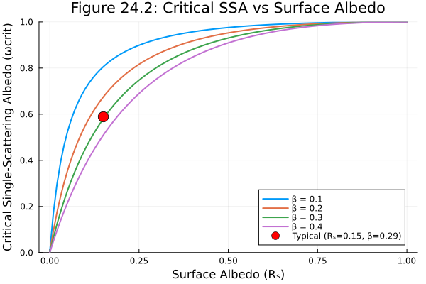
For the global mean surface albedo (Rs ≈ 0.15) and typical upscatter fraction (β ≈ 0.29), ωcrit ≈ 0.6. This means sulfate aerosols (ω ≈ 0.95) cause net cooling, while highly absorbing aerosols like black carbon can cause heating.
Figure 24.16: Cloud Albedo vs Optical Depth
Cloud albedo increases with optical depth according to the two-stream approximation (Eq. 24.38):
\[R_c = \frac{\tau_c}{\tau_c + \gamma}\]
where γ ≈ 7.7 for an asymmetry factor g = 0.85.
# Cloud albedo vs optical depth
τ_c_vals = 0.0:0.5:100.0
g = 0.85
γ = 2 / (sqrt(3) * (1 - g))

R_c_vals = [τ / (τ + γ) for τ in τ_c_vals]

p = plot(τ_c_vals, R_c_vals, xlabel = "Cloud Optical Depth (τc)",
    ylabel = "Cloud Albedo (Rc)", title = "Figure 24.16: Cloud Albedo vs Optical Depth",
    linewidth = 2, legend = false, xlim = (0, 100), ylim = (0, 1))

# Mark half-albedo point
scatter!(p, [γ], [0.5], markersize = 8, color = :red)
annotate!(p, γ + 5, 0.52, text("τc = γ ≈ 7.7\nRc = 0.5", 8, :left))

p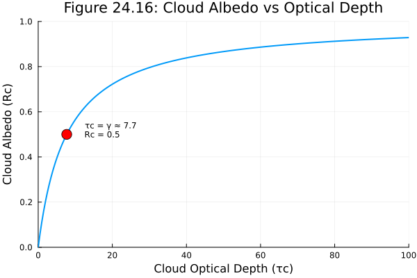
Figure 24.18: Twomey Susceptibility
The Twomey susceptibility quantifies how cloud albedo responds to changes in droplet number concentration (Eq. 24.41):
\[\frac{dR_c}{d \ln N} = \frac{R_c(1-R_c)}{3}\]
Maximum susceptibility occurs at R_c = 0.5.
R_c_vals = 0.0:0.01:1.0
S_vals = [R * (1 - R) / 3 for R in R_c_vals]

p = plot(R_c_vals, S_vals, xlabel = "Cloud Albedo (Rc)",
    ylabel = "Susceptibility dRc/d(ln N)",
    title = "Figure 24.18: Twomey Susceptibility",
    linewidth = 2, legend = false, xlim = (0, 1), ylim = (0, 0.1))

# Mark maximum
scatter!(p, [0.5], [0.5 * 0.5 / 3], markersize = 8, color = :red)
annotate!(p, 0.55, 0.085, text("Maximum at Rc = 0.5", 8, :left))

p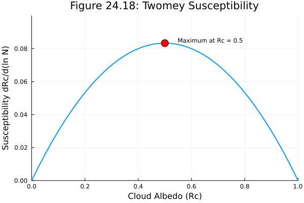
Figure 24.17: Cloud Albedo vs Cloud Droplet Number Concentration
Figure 24.17 shows cloud albedo as a function of cloud droplet number concentration at constant liquid water content (L = 0.3 g m⁻³). At constant liquid water content and cloud thickness, cloud albedo increases with increasing CDNC.
# Reproduce Figure 24.17: Cloud albedo vs CDNC
# Parameters from Figure 24.17 caption
L = 0.3e-3  # kg/m³ (0.3 g/m³)
ρ_w = 1000.0  # kg/m³
g = 0.85
γ = 2 / (sqrt(3) * (1 - g))

# Cloud thicknesses
h_vals = [50, 100, 500, 1500]  # meters

# CDNC range (cm⁻³)
N_cm3_range = 10.0:10.0:1000.0
N_range = N_cm3_range .* 1e6  # Convert to m⁻³

p = plot(xlabel = "Cloud Droplet Number Concentration (cm⁻³)",
    ylabel = "Cloud Albedo (Rᶜ)",
    title = "Figure 24.17: Cloud Albedo vs CDNC (L = 0.3 g m⁻³)",
    xscale = :log10, legend = :bottomright, ylim = (0, 1))

for h in h_vals
    τ_c_vals = [h * (9 * π * L^2 * N / (2 * ρ_w^2))^(1/3) for N in N_range]
    R_c_vals = [τ / (τ + γ) for τ in τ_c_vals]
    plot!(p, N_cm3_range, R_c_vals, label = "h = $h m", linewidth = 2)
end

p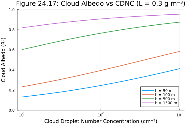
This figure demonstrates the potential of aerosols to affect climate indirectly. For a cloud 50 m thick, increasing CDNC from 100 to 1000 cm⁻³ nearly doubles cloud albedo (from ~0.2 to ~0.4).
Cloud Optical Depth Sensitivity
The relationship between cloud optical depth and cloud droplet number concentration (Eq. 24.36):
\[\tau_c = h \left(\frac{9\pi L^2 N}{2\rho_w^2}\right)^{1/3}\]
This shows that τ_c increases with N^(1/3), meaning a 30% increase in CDNC produces approximately a 9% increase in optical depth.
# Parameters from Figure 24.17
h = 500.0  # m (cloud thickness)
L = 0.3e-3  # kg/m³ (liquid water content)
ρ_w = 1000.0  # kg/m³

N_vals = 10e6:10e6:1000e6  # m⁻³

τ_c_vals = [h * (9 * π * L^2 * N / (2 * ρ_w^2))^(1/3) for N in N_vals]

# Convert to cm⁻³ for plotting
N_cm3 = N_vals ./ 1e6

p = plot(N_cm3, τ_c_vals, xlabel = "Cloud Droplet Number (cm⁻³)",
    ylabel = "Cloud Optical Depth (τc)",
    title = "Cloud Optical Depth vs CDNC (h=500m, L=0.3 g/m³)",
    linewidth = 2, legend = false, xscale = :log10)

p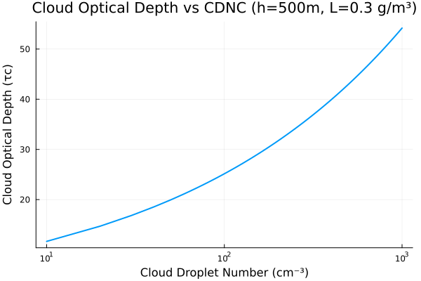
Indirect Aerosol Forcing
The change in shortwave forcing due to aerosol-induced changes in cloud albedo (Eq. 24.43):
\[\Delta F_c = -F_0 \cdot A_c \cdot T_a^2 \cdot \Delta R_c\]
where ΔR_c depends on the fractional change in CDNC through the Twomey relationship.
# Calculate forcing for different fractional changes in N
F_0 = 1370.0  # W/m²
A_c = 0.6     # Cloud fraction
T_a = 0.76   # Atmospheric transmittance
R_c = 0.5    # Cloud albedo

Δln_N_vals = 0.0:0.01:0.5  # Fractional change in N

ΔR_c_vals = [R_c * (1 - R_c) / 3 * Δln_N for Δln_N in Δln_N_vals]
ΔF_c_vals = [-F_0 * A_c * T_a^2 * ΔR_c for ΔR_c in ΔR_c_vals]

# Convert to percentage for x-axis
percent_change = (exp.(Δln_N_vals) .- 1) .* 100

p = plot(percent_change, ΔF_c_vals, xlabel = "Percent Increase in CDNC (%)",
    ylabel = "ΔFc (W/m²)",
    title = "Indirect Aerosol Forcing vs CDNC Change",
    linewidth = 2, legend = false)

# Mark 30% increase point
idx_30 = argmin(abs.(percent_change .- 30))
scatter!(p, [percent_change[idx_30]], [ΔF_c_vals[idx_30]], markersize = 8, color = :red)
annotate!(p, 35, ΔF_c_vals[idx_30] - 1,
    text("30% increase\n≈ $(round(ΔF_c_vals[idx_30], digits=1)) W/m²", 8, :left))

p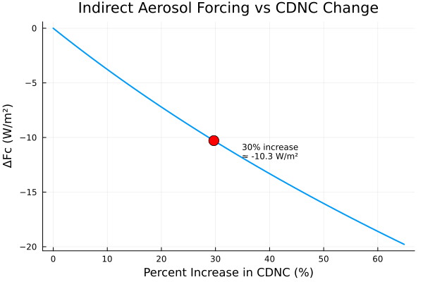
Physical Interpretation
Direct Aerosol Effects
The direct radiative forcing of aerosols depends on three key properties:
Single-scattering albedo (ω): The fraction of extinction due to scattering vs absorption. Pure sulfate aerosols have ω ≈ 0.95-1.0, while black carbon has ω ≈ 0.2-0.3.
Upscatter fraction (β): The fraction of scattered radiation directed upward, which depends on particle size and solar zenith angle. Typical values range from 0.1-0.4.
Aerosol optical depth (τ): The integrated extinction through the aerosol layer. Typical tropospheric values are τ ≈ 0.1.
Indirect Aerosol Effects
The first indirect effect (Twomey effect) operates through this chain:
- Increased aerosol concentration → More CCN
- More CCN → More cloud droplets for fixed liquid water
- More droplets → Smaller droplet size
- Smaller droplets → Higher cloud optical depth
- Higher optical depth → Higher cloud albedo
- Higher albedo → More reflected sunlight (cooling)
The second indirect effect (cloud lifetime effect) involves precipitation suppression, which is not implemented in this module.
References
- Seinfeld, J. H., and Pandis, S. N. (2006). Atmospheric Chemistry and Physics, Chapter 24.
- Charlson, R. J., et al. (1992). Climate forcing by anthropogenic aerosols. Science, 255(5043), 423-430.
- Twomey, S. (1977). The influence of pollution on the shortwave albedo of clouds. J. Atmos. Sci., 34, 1149-1152.
- Haywood, J. M., and Shine, K. P. (1995). The effect of anthropogenic sulfate and soot aerosol on the clear sky planetary radiation budget. Geophys. Res. Lett., 22(5), 603-606.