Aerosol Population Dynamics
Overview
This module implements aerosol population dynamics equations from Chapter 13 of Seinfeld & Pandis (2006), including condensational growth, Brownian coagulation, and the general dynamic equation.
Reference: Seinfeld, J. H. and Pandis, S. N. (2006) Atmospheric Chemistry and Physics: From Air Pollution to Climate Change, 2nd Edition, Chapter 13, pp. 588-627.
Aerosol.AerosolDynamics — Function
AerosolDynamics(; name=:AerosolDynamics)A combined system for modeling aerosol population dynamics including condensation growth and coagulation processes.
Reference: Seinfeld, J. H. and Pandis, S. N. (2006) Atmospheric Chemistry and Physics, 2nd Edition, Chapter 13.
This system provides:
- Condensation growth rate calculation
- Brownian coagulation coefficient (Fuchs form)
- Monodisperse coagulation dynamics
The General Dynamic Equation (Eq. 13.86) combines these processes:
$\frac{\partial n(v,t)}{\partial t} = \left(\frac{\partial n}{\partial t}\right)_{coag} + \left(\frac{\partial n}{\partial t}\right)_{cond} + J_0\delta(v-v_0) + S(v) - R(v)$
Aerosol.DiameterGrowthRate — Function
DiameterGrowthRate(; name=:DiameterGrowthRate)Compute the diameter growth rate due to condensation in the continuum regime.
Reference: Seinfeld, J. H. and Pandis, S. N. (2006) Atmospheric Chemistry and Physics, 2nd Edition, Chapter 13, Eq. 13.11-13.13.
The diameter growth rate is given by:
$I_D = \frac{dD_p}{dt} = \frac{4 D_i M_i}{R T D_p \rho_p} (p_i - p_{eq,i})$
In the continuum regime with constant supersaturation (A = constant), this simplifies to:
$I_D = \frac{A}{D_p}$
where $A = \frac{4 D_i M_i}{R T \rho_p} (p_i - p_{eq,i})$.
Aerosol.BrownianCoagulationCoefficient — Function
BrownianCoagulationCoefficient(; name=:BrownianCoagulationCoefficient)Compute the Brownian coagulation coefficient using the Fuchs form, which is valid across the continuum, transition, and free-molecular regimes.
Reference: Seinfeld, J. H. and Pandis, S. N. (2006) Atmospheric Chemistry and Physics, 2nd Edition, Chapter 13, Table 13.1.
The Fuchs form of the coagulation coefficient is:
$K_{12} = 2\pi(D_1 + D_2)(D_{p1} + D_{p2}) \left( \frac{D_{p1} + D_{p2}}{D_{p1} + D_{p2} + 2\sqrt{g_1^2 + g_2^2}} + \frac{8(D_1 + D_2)}{\sqrt{\bar{c}_1^2 + \bar{c}_2^2}(D_{p1} + D_{p2})} \right)^{-1}$
where:
- $D_i = \frac{k T C_c}{3\pi\mu D_{pi}}$ is the Brownian diffusion coefficient
- $\bar{c}_i = \sqrt{\frac{8 k T}{\pi m_i}}$ is the mean thermal velocity
- $\ell_i = \frac{8 D_i}{\pi \bar{c}_i}$ is the particle mean free path
- $g_i = \frac{1}{3 D_{pi} \ell_i}\left[(D_{pi} + \ell_i)^3 - (D_{pi}^2 + \ell_i^2)^{3/2}\right] - D_{pi}$
Aerosol.MonodisperseCoagulation — Function
MonodisperseCoagulation(; name=:MonodisperseCoagulation)Model the evolution of total aerosol number concentration for a monodisperse aerosol undergoing Brownian coagulation with a constant coagulation coefficient.
Reference: Seinfeld, J. H. and Pandis, S. N. (2006) Atmospheric Chemistry and Physics, 2nd Edition, Chapter 13, Eq. 13.65-13.67.
The governing equation is:
$\frac{dN}{dt} = -\frac{1}{2} K N^2(t)$
with analytical solution:
$N(t) = \frac{N_0}{1 + t/\tau_c}$
where $\tau_c = \frac{2}{K N_0}$ is the characteristic coagulation time.
Aerosol.DiscreteCoagulation — Function
DiscreteCoagulation(n_bins::Int; name=:DiscreteCoagulation)Model the discrete coagulation equation for a monodisperse initial distribution with constant coagulation coefficient.
Reference: Seinfeld, J. H. and Pandis, S. N. (2006) Atmospheric Chemistry and Physics, 2nd Edition, Chapter 13, Eq. 13.59, 13.71.
The discrete coagulation equation for k-mers is:
$\frac{dN_k}{dt} = \frac{1}{2} \sum_{j=1}^{k-1} K_{j,k-j} N_j N_{k-j} - N_k \sum_{j=1}^{\infty} K_{kj} N_j$
For a constant coagulation coefficient K and monodisperse initial condition (all particles initially monomers), the analytical solution is:
$N_k(t) = \frac{N_0 (t/\tau_c)^{k-1}}{[1 + t/\tau_c]^{k+1}}$
Arguments:
n_bins::Int: Number of size bins (k-mer sizes to track)
Implementation
Condensational Growth
The diameter growth rate due to condensation is given by Eq. 13.11:
\[I_D = \frac{dD_p}{dt} = \frac{4 D_i M_i}{R T D_p \rho_p} (p_i - p_{eq,i})\]
In the continuum regime with constant supersaturation, this simplifies to Eq. 13.13:
\[I_D = \frac{A}{D_p}\]
where $A = \frac{4 D_i M_i}{R T \rho_p} (p_i - p_{eq,i})$ is the growth parameter.
The analytical solution for particle diameter evolution (Eq. 13.21) is:
\[D_p^2 = D_{p0}^2 + 2At\]
State Variables
using DataFrames, ModelingToolkit, Symbolics, DynamicQuantities
using Aerosol

sys = DiameterGrowthRate()

vars = unknowns(sys)
DataFrame(
    :Name => [string(Symbolics.tosymbol(v, escape = false)) for v in vars],
    :Units => [dimension(ModelingToolkit.get_unit(v)) for v in vars],
    :Description => [ModelingToolkit.getdescription(v) for v in vars]
)| Row | Name | Units | Description |
|---|---|---|---|
| String | Dimensio… | String | |
| 1 | D_p | m | Particle diameter |
| 2 | A | m² s⁻¹ | Growth parameter |
| 3 | I_D | m s⁻¹ | Diameter growth rate |
Parameters
params = parameters(sys)
DataFrame(
    :Name => [string(Symbolics.tosymbol(p, escape = false)) for p in params],
    :Units => [dimension(ModelingToolkit.get_unit(p)) for p in params],
    :Description => [ModelingToolkit.getdescription(p) for p in params]
)| Row | Name | Units | Description |
|---|---|---|---|
| String | Dimensio… | String | |
| 1 | D_diff | m² s⁻¹ | Diffusion coefficient of condensing species |
| 2 | M_i | kg mol⁻¹ | Molecular weight of condensing species |
| 3 | Δp | m⁻¹ kg s⁻² | Vapor pressure difference (p_i - p_eq) |
| 4 | T | K | Temperature |
| 5 | R_gas | m² kg s⁻² K⁻¹ mol⁻¹ | Universal gas constant |
| 6 | ρ_p | m⁻³ kg | Particle density |
Equations
equations(sys)3-element Vector{Symbolics.Equation}:
Differential(t, 1)(D_p(t)) ~ I_D(t)
A(t) ~ (4D_diff*M_i*Δp) / (R_gas*T*ρ_p)
I_D(t) ~ A(t) / D_p(t)Analysis
Particle Growth Curves (Figure 13.2)
This figure shows the growth of particles of different initial sizes due to condensation. Smaller particles grow more slowly in diameter because the growth rate is inversely proportional to particle size.
using Plots
using OrdinaryDiffEq
using ModelingToolkit: t

sys = DiameterGrowthRate()
compiled_sys = mtkcompile(sys)

# Parameters from Figure 13.2
D_diff = 0.1e-4  # m²/s
M_i = 0.1        # kg/mol (100 g/mol)
Δp = 1e-4        # Pa (~1 ppb at 1 atm)
T_val = 298.0    # K
ρ_p = 1000.0     # kg/m³

# Initial diameters
D_p0_values = [0.2e-6, 0.5e-6, 2.0e-6]  # 0.2, 0.5, 2 μm

tspan = (0.0, 1200.0)  # 20 minutes

plt = plot(
    xlabel = "Time (minutes)",
    ylabel = "Diameter (μm)",
    title = "Particle Growth by Condensation",
    legend = :topleft
)

for D_p0 in D_p0_values
    prob = ODEProblem(
        compiled_sys,
        [compiled_sys.D_p => D_p0],
        tspan,
        [
            compiled_sys.D_diff => D_diff,
            compiled_sys.M_i => M_i,
            compiled_sys.Δp => Δp,
            compiled_sys.T => T_val,
            compiled_sys.ρ_p => ρ_p
        ]
    )
    sol = solve(prob)

    plot!(plt, sol.t ./ 60, sol[compiled_sys.D_p] .* 1e6,
        label = "D₀ = $(D_p0 * 1e6) μm")
end

plt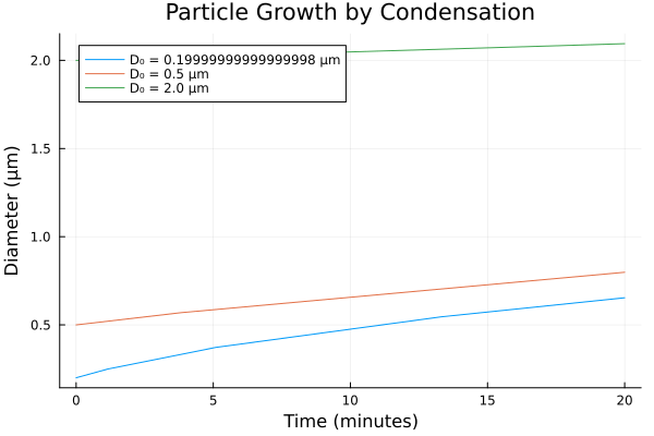
Brownian Coagulation Coefficient
The Brownian coagulation coefficient determines how fast particles of different sizes collide and stick together. The Fuchs form (Table 13.1) provides an interpolation formula that is valid across all regimes:
sys_coag = BrownianCoagulationCoefficient()

# Show the coagulation coefficient equations
equations(sys_coag)
15-element Vector{Symbolics.Equation}:
m_1(t) ~ (1//6)*(D_p1^3)*π_val*ρ_p
m_2(t) ~ (1//6)*(D_p2^3)*π_val*ρ_p
Kn_1(t) ~ (2λ_air) / D_p1
Kn_2(t) ~ (2λ_air) / D_p2
C_c1(t) ~ 1 + Kn_1(t)*(1.257 + 0.4exp(-1.1 / Kn_1(t)))
C_c2(t) ~ 1 + Kn_2(t)*(1.257 + 0.4exp(-1.1 / Kn_2(t)))
D_1(t) ~ (C_c1(t)*T*k_B) / (3D_p1*μ*π_val)
D_2(t) ~ (C_c2(t)*T*k_B) / (3D_p2*μ*π_val)
c_bar_1(t) ~ sqrt((8T*k_B) / (m_1(t)*π_val))
c_bar_2(t) ~ sqrt((8T*k_B) / (m_2(t)*π_val))
ℓ_1(t) ~ (8D_1(t)) / (c_bar_1(t)*π_val)
ℓ_2(t) ~ (8D_2(t)) / (c_bar_2(t)*π_val)
g_1(t) ~ -D_p1 + (-((D_p1^2 + ℓ_1(t)^2)^1.5) + (D_p1 + ℓ_1(t))^3) / (3D_p1*ℓ_1(t))
g_2(t) ~ -D_p2 + (-((D_p2^2 + ℓ_2(t)^2)^1.5) + (D_p2 + ℓ_2(t))^3) / (3D_p2*ℓ_2(t))
K_12(t) ~ (2(D_1(t) + D_2(t))*(D_p1 + D_p2)*π_val) / ((8(D_1(t) + D_2(t))) / ((D_p1 + D_p2)*sqrt(c_bar_1(t)^2 + c_bar_2(t)^2)) + (D_p1 + D_p2) / (D_p1 + D_p2 + 2sqrt(g_1(t)^2 + g_2(t)^2)))The coagulation coefficient depends strongly on particle size, with a minimum for particles of similar size in the transition regime and higher values for either very small particles (free molecular regime) or very large particles (continuum regime), or for particles of very different sizes.
Monodisperse Coagulation Dynamics (Eq. 13.65-13.67)
For a monodisperse aerosol with constant coagulation coefficient, the total number concentration evolves according to:
\[\frac{dN}{dt} = -\frac{1}{2} K N^2\]
with analytical solution:
\[N(t) = \frac{N_0}{1 + t/\tau_c}\]
where $\tau_c = \frac{2}{K N_0}$ is the characteristic coagulation time.
sys_mono = MonodisperseCoagulation()
compiled_mono = mtkcompile(sys_mono)

N_0_val = 1e12  # 10⁶ cm⁻³ = 10¹² m⁻³
K_val = 1e-15   # m³/s
τ_c = 2 / (K_val * N_0_val)

prob_mono = ODEProblem(
    compiled_mono,
    [compiled_mono.N => N_0_val],
    (0.0, 5 * τ_c),
    [
        compiled_mono.K => K_val,
        compiled_mono.N_0 => N_0_val
    ]
)
sol_mono = solve(prob_mono)

# Plot numerical vs analytical solution
t_plot = range(0, 5 * τ_c, length = 100)
N_analytical = N_0_val ./ (1 .+ t_plot ./ τ_c)

plot(sol_mono.t ./ τ_c, sol_mono[compiled_mono.N] ./ N_0_val,
    label = "Numerical", lw = 2,
    xlabel = "t / τc",
    ylabel = "N / N₀",
    title = "Monodisperse Coagulation (Eq. 13.66)")
plot!(t_plot ./ τ_c, N_analytical ./ N_0_val,
    label = "Analytical: N₀/(1 + t/τc)", ls = :dash, lw = 2)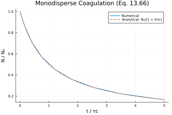
Characteristic Coagulation Time
The characteristic coagulation time depends on both the coagulation coefficient and the initial number concentration. For atmospheric aerosols:
| N₀ (m⁻³) | K (m³/s) | τc | Physical Interpretation |
|---|---|---|---|
| 10¹⁰ | 10⁻¹⁵ | ~55 hours | Clean background |
| 10¹² | 10⁻¹⁵ | ~33 minutes | Polluted urban |
| 10¹⁴ | 10⁻¹⁵ | ~20 seconds | Fresh emissions |
Discrete Coagulation (Eq. 13.59, 13.71)
For an initially monodisperse aerosol, the evolution of k-mer concentrations follows the discrete coagulation equation. The analytical solution for constant K is:
\[N_k(t) = \frac{N_0 (t/\tau_c)^{k-1}}{[1 + t/\tau_c]^{k+1}}\]
n_bins = 8
sys_discrete = DiscreteCoagulation(n_bins)
compiled_discrete = mtkcompile(sys_discrete)

# Initially all monomers
u0 = [compiled_discrete.N[1] => N_0_val]
for k in 2:n_bins
    push!(u0, compiled_discrete.N[k] => 0.0)
end

prob_discrete = ODEProblem(
    compiled_discrete,
    u0,
    (0.0, 3 * τ_c),
    [
        compiled_discrete.K => K_val,
        compiled_discrete.N_0 => N_0_val
    ]
)
sol_discrete = solve(prob_discrete)

# Plot k-mer evolution
plt_kmer = plot(
    xlabel = "t / τc",
    ylabel = "Nk / N₀",
    title = "Evolution of k-mer Concentrations (Eq. 13.71)",
    legend = :topright
)

for k in 1:min(5, n_bins)
    plot!(plt_kmer, sol_discrete.t ./ τ_c,
        sol_discrete[compiled_discrete.N[k]] ./ N_0_val,
        label = "N$k", lw = 2)
end

plt_kmer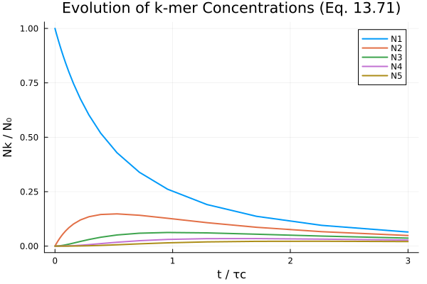
Conservation Properties (Table 13.4)
Coagulation conserves total aerosol volume (mass) while decreasing total number. Condensation conserves number while increasing volume. This is verified numerically:
| Process | Number (N) | Volume/Mass (V) |
|---|---|---|
| Coagulation | Decreases | Conserved |
| Condensation | Conserved | Increases |
| Coag + Cond | Decreases | Increases |
| Nucleation | Increases | Increases |