VBS: Volatility Basis Set (VBS) model that deals with the partitioning of Secondary Organic Aerosol (SOA)
Model
This is an implementation of the model to simulate the behavior of semivolatile organic compounds in the atmosphere, as described in Donahue et al. (2006):
We can create an instance of the model in the following manner. Ci is the input of the function, which is the organic compound concentration in all phases (air and aerosol phase), values were read from the original Figure 1.(a):
using Aerosol
using NonlinearSolve, ModelingToolkit

Ci = [2.5, 1.8, 4.0, 4.0, 5.8, 4.8, 6.3, 8.0]
ns = VBS(Ci)
We could solve and visualize the results with the following codes, Let's try reproducing Figure 1.(a):
simplens = mtkcompile(ns)
guess = [29] # initial guess of the C_OA, the total organic compound in aerosol phase
prob = NonlinearProblem(simplens, guess, [])
sol = solve(prob, TrustRegion())
┌ Warning: `SciMLBase.NonlinearProblem(sys, u0, p; kw...)` is deprecated. Use `SciMLBase.NonlinearProblem(sys, merge(if isempty(u0)
│ Dict()
│ else
│ Dict(unknowns(sys) .=> u0)
│ end, if isempty(p)
│ Dict()
│ else
│ Dict(parameters(sys) .=> p)
│ end))`
│ instead.
└ @ ModelingToolkitBase ~/.julia/packages/ModelingToolkitBase/PHXso/src/deprecations.jl:141Figure 1.(a) shows a partitioning in ideal situations that compounds are distributed without any potential effects. The green part is the concentration of organic compounds in aerosol phase and white part is the concentration in gas phase.
using Plots
p1 = begin
    x = log10.([0.01, 0.1, 1, 10, 100, 1000, 10000, 100000])
    p = bar(x, Ci, label = "total", color = :white)
    bar!(x, sol[simplens.ξ] .* Ci, label = "condensed-phase", color = :green)
    ylabel!("Organic Mass, μg/m³")
    xlabel!("log10(C*)")
    title!("Typical Ambient Partitioning")
end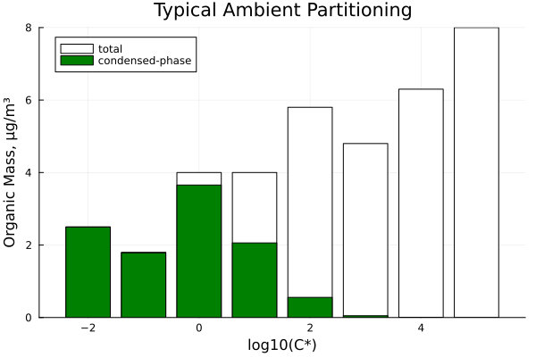
Let's try reproducing Figure 1.(b): Semi-volatile emissions as they might appear near the output of a primarysource, before substantial dilution into the background atmosphere (only enough dilution to cool the emissions to ambient temperatureis assumed). The high loading leads to partitioning well into the highC* end of the distribution, as shown in brown. Note the scale oftheyaxis (mg/m³).
Ci_2 = [0.4, 0.8, 1.25, 1.7, 2.1, 2.5, 3, 3.4] .* 1000 # The unit of Ci is μg/m³, and the values read from the original Figure 1(b) are in units of mg/m³
ns2 = VBS(Ci_2)
simplens2 = mtkcompile(ns2)
prob2 = NonlinearProblem(simplens2, [10000], [])
sol2 = solve(prob2, TrustRegion())
p2 = begin
    x = log10.([0.01, 0.1, 1, 10, 100, 1000, 10000, 100000])
    p = bar(x, Ci_2, label = "total", color = :white)
    bar!(x, sol2[simplens2.ξ] .* Ci_2, label = "condensed-phase", color = :red)
    ylabel!("Organic Mass, mg/m³")
    xlabel!("log10(C*)")
    title!("Cooled Fresh Emissions")
end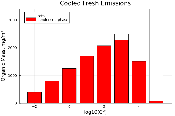
Let's try reproducing Figure 1.(c): The effect of dilution by pure air on the emissionsdepicted above. The dilution factor of 1000 is indicated with a horizontal black arrow. Dilution by a factor of 1000 reduces the aerosolmass by a factor of 4000 because of repartitioning into the vapor phase
Ci_3 = [0.4, 0.8, 1.25, 1.7, 2.1, 2.5, 3, 3.4]
simplens3 = mtkcompile(VBS(Ci_3))
sol3 = solve(NonlinearProblem(simplens3, [10], []), TrustRegion())
p3 = begin
    x = log10.([0.01, 0.1, 1, 10, 100, 1000, 10000, 100000])
    p = bar(x, Ci_3, label = "total", color = :white)
    bar!(x, sol3[simplens3.ξ] .* Ci_3, label = "condensed-phase", color = :red)
    ylabel!("Organic Mass, μg/m³")
    xlabel!("log10(C*)")
    title!("Diluted Emissions (dilution factor = 1000)")
end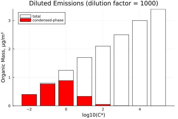
Let's try reproducing Figure 1.(d): The effect of dilution, as depicted in panel b above but nowinto background air represented in panel a above. The partitioning of the background organic material and the fresh emissions are keptseparate, in green and brown, only for illustrative purposes. The vapor portions of the background and the fresh emissions are alsoseparated, though each is shown with a white bar.
p4 = begin
    x = log10.([0.4, 0.8, 1.25, 1.7, 2.1, 2.5, 3, 3.4])
    Ci_sum = Ci .+ Ci_3
    p = bar(x, Ci_sum, label = "total", color = :white)
    both = sol[simplens.ξ] .* Ci .+ sol3[simplens3.ξ] .* Ci_3
    bar!(x, both, label = "diluted emission", color = :red)
    bar!(x, sol[simplens.ξ] .* Ci, label = "background", color = :green)
    ylabel!("Organic Mass, μg/m³")
    xlabel!("log10(C*)")
    title!("Emission & Background Mixed")
end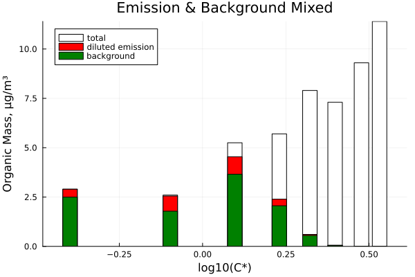
Temperature dependence
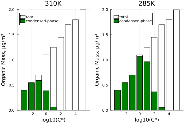
Temperature dependence was taken into consideration. A basis set of saturation concentrations (ranging from 1 ng to 100 mg at 300 K) changes with temperature according to the Clausius Clapeyron equation. Let's try reproducing Figure 2:
Ci_t = [0.4, 0.55, 0.7, 1.1, 1.25, 1.45, 1.7, 1.8, 2] # values were read from the original Figure
ns_t = VBS(Ci_t, [0.001, 0.01, 0.1, 1, 10, 100, 1000, 10000, 100000]) # The second input of the VBS function is different basic set at standard temperatures, ranging from 1 ng to 100 mg at 300 K
simplens_t = mtkcompile(ns_t)
prob_310 = NonlinearProblem(simplens_t, [29], [simplens_t.T=>310]) # Temperature is an adjustable parameter in the model.
prob_285 = NonlinearProblem(simplens_t, [29], [simplens_t.T=>285])
sol_310 = solve(prob_310, TrustRegion())
sol_285 = solve(prob_285, TrustRegion())

# Helpful visualize function
function pl_t(sol, simplens_t, string::String)
    x = log10.([0.001, 0.01, 0.1, 1, 10, 100, 1000, 10000, 100000])
    p = bar(x, Ci_t, label = "total", color = :white)
    bar!(x, sol[simplens_t.ξ] .* Ci_t, label = "condensed-phase", color = :green)
    ylabel!("Organic Mass, μg/m³")
    xlabel!("log10(C*)")
    title!(string)
end
plot(pl_t(sol_310, simplens_t, "310K"), pl_t(sol_285, simplens_t, "285K"), layout = (1, 2))