Single Particle Dynamics
Overview
This module implements equations for the dynamics of single aerosol particles, covering the fundamental physics that govern particle motion, transport, and interactions with gas molecules. These equations are essential for understanding aerosol behavior in the atmosphere, including sedimentation, diffusion, and electrical migration.
Reference: Seinfeld, J. H. and Pandis, S. N. (2006) Atmospheric Chemistry and Physics: From Air Pollution to Climate Change, 2nd Edition, Chapter 9: Dynamics of Single Aerosol Particles, pp. 396-433. John Wiley & Sons, Inc.
Aerosol.SingleParticleDynamics — Function
SingleParticleDynamics(; name=:SingleParticleDynamics)Comprehensive component combining all single particle dynamics equations.
Reference: Seinfeld, J. H. and Pandis, S. N. (2006) Atmospheric Chemistry and Physics, 2nd Edition, Chapter 9: Dynamics of Single Aerosol Particles.
This component calculates key aerosol particle properties:
- Mean free path of air (Eq. 9.6)
- Knudsen number (Eq. 9.1)
- Cunningham slip correction factor (Eq. 9.34)
- Terminal settling velocity (Eq. 9.42)
- Relaxation time (Eq. 9.38)
- Brownian diffusion coefficient (Eq. 9.73)
- Particle mobility (Eq. 9.78)
- Mean thermal speed (Eq. 9.87)
- Particle mean free path (Eq. 9.89)
- Aerodynamic diameter (Eq. 9.110)
Aerosol.MeanFreePath — Function
MeanFreePath(; name=:MeanFreePath)Component for calculating the mean free path of air molecules.
Reference: Seinfeld, J. H. and Pandis, S. N. (2006) Atmospheric Chemistry and Physics, 2nd Edition, Chapter 9, Eq. 9.6.
The mean free path is calculated from:
\[\lambda = \frac{2\mu}{p\sqrt{8M/(\pi R T)}}\]
where μ is dynamic viscosity, p is pressure, M is molecular weight, R is the gas constant, and T is temperature.
Aerosol.SlipCorrection — Function
SlipCorrection(; name=:SlipCorrection)Component for calculating the Cunningham slip correction factor.
Reference: Seinfeld, J. H. and Pandis, S. N. (2006) Atmospheric Chemistry and Physics, 2nd Edition, Chapter 9, Eq. 9.34.
The slip correction factor accounts for noncontinuum effects when the particle size approaches the mean free path of gas molecules:
\[C_c = 1 + \frac{2\lambda}{D_p}\left[A_1 + A_2 \exp\left(-\frac{A_3 D_p}{2\lambda}\right)\right]\]
where the constants A₁ = 1.257, A₂ = 0.4, A₃ = 1.1 are from Allen & Raabe (1982).
Aerosol.SettlingVelocity — Function
SettlingVelocity(; name=:SettlingVelocity)Component for calculating particle terminal settling velocity and relaxation time.
Reference: Seinfeld, J. H. and Pandis, S. N. (2006) Atmospheric Chemistry and Physics, 2nd Edition, Chapter 9, Eqs. 9.38, 9.42.
The terminal settling velocity is given by:
\[v_t = \frac{D_p^2 \rho_p g C_c}{18\mu}\]
The relaxation time (time constant for velocity adjustment) is:
\[\tau = \frac{\rho_p D_p^2 C_c}{18\mu}\]
Aerosol.BrownianDiffusion — Function
BrownianDiffusion(; name=:BrownianDiffusion)Component for calculating Brownian diffusion properties of aerosol particles.
Reference: Seinfeld, J. H. and Pandis, S. N. (2006) Atmospheric Chemistry and Physics, 2nd Edition, Chapter 9, Eqs. 9.73, 9.78, 9.87, 9.89.
The Stokes-Einstein-Sutherland relation gives the diffusion coefficient:
\[D = \frac{k T C_c}{3 \pi \mu D_p}\]
The particle mobility is:
\[B = \frac{C_c}{3 \pi \mu D_p}\]
The mean thermal speed of the particle is:
\[\bar{c}_p = \sqrt{\frac{8 k T}{\pi m_p}}\]
The particle mean free path is derived from D = ½ c̄p λp (Eq. 9.88):
\[\lambda_p = \frac{2D}{\bar{c}_p}\]
Aerosol.ParticleMobility — Function
ParticleMobility(; name=:ParticleMobility)Component for calculating particle mechanical mobility.
Reference: Seinfeld, J. H. and Pandis, S. N. (2006) Atmospheric Chemistry and Physics, 2nd Edition, Chapter 9, Eq. 9.78.
The particle mobility relates external force to drift velocity:
\[B = \frac{C_c}{3 \pi \mu D_p}\]
With the Einstein relation connecting mobility to diffusion:
\[D = B k T\]
Aerosol.ElectricalMobility — Function
ElectricalMobility(; name=:ElectricalMobility)Component for calculating electrical mobility and migration velocity.
Reference: Seinfeld, J. H. and Pandis, S. N. (2006) Atmospheric Chemistry and Physics, 2nd Edition, Chapter 9, Eqs. 9.49, 9.50, 9.51.
The electrical mobility relates particle velocity to electric field strength:
\[B_e = \frac{q C_c}{3 \pi \mu D_p}\]
The migration velocity in an electric field E is:
\[v_e = B_e E\]
Aerosol.StokesNumber — Function
StokesNumber(; name=:StokesNumber)Component for calculating Stokes number and stop distance.
Reference: Seinfeld, J. H. and Pandis, S. N. (2006) Atmospheric Chemistry and Physics, 2nd Edition, Chapter 9, Eqs. 9.98, 9.101.
The stop distance is the distance a particle travels before coming to rest:
\[s_p = \tau U\]
The Stokes number characterizes particle inertia relative to flow:
\[St = \frac{\tau u_0}{L} = \frac{D_p^2 \rho_p C_c u_0}{18 \mu L}\]
When St ≫ 1, particles cannot follow fluid streamlines (inertial impaction). When St ≪ 1, particles follow fluid motion closely.
Aerosol.AerodynamicDiameter — Function
AerodynamicDiameter(; name=:AerodynamicDiameter)Component for calculating equivalent particle diameters.
Reference: Seinfeld, J. H. and Pandis, S. N. (2006) Atmospheric Chemistry and Physics, 2nd Edition, Chapter 9, Eqs. 9.102, 9.106, 9.108, 9.110, 9.114.
The volume equivalent diameter is the diameter of a sphere with the same volume:
\[D_{ve} = \left(\frac{6 V_p}{\pi}\right)^{1/3}\]
The aerodynamic diameter is defined for a sphere of unit density (1000 kg/m³) with the same settling velocity:
\[D_{ca} = D_p \sqrt{\frac{\rho_p}{\rho_p^\circ}} \sqrt{\frac{C_c(D_p)}{C_c(D_{ca})}}\]
In the continuum regime (large particles), this simplifies to:
\[D_{ca} \approx D_p \sqrt{\frac{\rho_p}{\rho_p^\circ}}\]
The electrical mobility equivalent diameter relates to mobility measurement:
\[D_{em} = D_{ve} \chi \frac{C_c(D_{em})}{C_c(D_{ve})}\]
Implementation
The implementation provides several components that can be used individually or combined through the comprehensive SingleParticleDynamics component.
Key Physical Quantities
The implementation calculates the following key quantities:
| Quantity | Symbol | Equation | Description |
|---|---|---|---|
| Mean free path | λ | Eq. 9.6 | Average distance traveled by air molecules between collisions |
| Knudsen number | Kn | Eq. 9.1 | Ratio of mean free path to particle diameter |
| Slip correction | Cc | Eq. 9.34 | Correction for non-continuum effects |
| Relaxation time | τ | Eq. 9.38 | Time constant for velocity adjustment |
| Terminal velocity | vt | Eq. 9.42 | Steady-state settling velocity |
| Diffusion coefficient | D | Eq. 9.73 | Brownian diffusivity |
| Particle mobility | B | Eq. 9.78 | Mechanical mobility |
State Variables
using Aerosol, ModelingToolkit, DataFrames, DynamicQuantities

sys = SingleParticleDynamics()
vars = unknowns(sys)
DataFrame(
    :Name => [string(v) for v in vars],
    :Units => [string(ModelingToolkit.get_unit(v)) for v in vars],
    :Description => [ModelingToolkit.getdescription(v) for v in vars]
)| Row | Name | Units | Description |
|---|---|---|---|
| String | String | String | |
| 1 | λ(t) | 1.0 m | Mean free path of air |
| 2 | Kn(t) | 1.0 | Knudsen number (dimensionless) |
| 3 | C_c(t) | 1.0 | Cunningham slip correction factor (dimensionless) |
| 4 | m_p(t) | 1.0 kg | Particle mass |
| 5 | τ(t) | 1.0 s | Relaxation time |
| 6 | v_t(t) | 1.0 m s⁻¹ | Terminal settling velocity |
| 7 | D_B(t) | 1.0 m² s⁻¹ | Brownian diffusion coefficient |
| 8 | B(t) | 1.0 kg⁻¹ s | Particle mobility |
| 9 | c_p(t) | 1.0 m s⁻¹ | Mean thermal speed of particle |
| 10 | λ_p(t) | 1.0 m | Particle mean free path |
| 11 | D_ca(t) | 1.0 m | Aerodynamic diameter (continuum limit) |
Parameters
params = parameters(sys)
DataFrame(
    :Name => [string(p) for p in params],
    :Units => [string(ModelingToolkit.get_unit(p)) for p in params],
    :Description => [ModelingToolkit.getdescription(p) for p in params]
)| Row | Name | Units | Description |
|---|---|---|---|
| String | String | String | |
| 1 | μ | 1.0 m⁻¹ kg s⁻¹ | Dynamic viscosity of air |
| 2 | M_air | 1.0 kg mol⁻¹ | Molecular weight of air |
| 3 | T | 1.0 K | Temperature |
| 4 | π_val | 1.0 | Pi (dimensionless) |
| 5 | R | 1.0 m² kg s⁻² K⁻¹ mol⁻¹ | Molar gas constant |
| 6 | P | 1.0 m⁻¹ kg s⁻² | Pressure |
| 7 | D_p | 1.0 m | Particle diameter |
| 8 | A1 | 1.0 | Slip correction constant A1 (dimensionless) |
| 9 | A2 | 1.0 | Slip correction constant A2 (dimensionless) |
| 10 | A3 | 1.0 | Slip correction constant A3 (dimensionless) |
| 11 | ρ_p | 1.0 m⁻³ kg | Particle density |
| 12 | g | 1.0 m s⁻² | Gravitational acceleration |
| 13 | k_B | 1.0 m² kg s⁻² K⁻¹ | Boltzmann constant |
| 14 | ρ_p0 | 1.0 m⁻³ kg | Reference density (1 g/cm³) |
Equations
equations(sys)11-element Vector{Symbolics.Equation}:
λ(t) ~ (2μ) / (P*sqrt((8M_air) / (R*T*π_val)))
Kn(t) ~ (2λ(t)) / D_p
C_c(t) ~ 1 + (A1 + A2*exp((-A3) / Kn(t)))*Kn(t)
m_p(t) ~ (1//6)*(D_p^3)*π_val*ρ_p
τ(t) ~ (C_c(t)*(D_p^2)*ρ_p) / (18μ)
v_t(t) ~ g*τ(t)
D_B(t) ~ (C_c(t)*T*k_B) / (3D_p*μ*π_val)
B(t) ~ C_c(t) / (3D_p*μ*π_val)
c_p(t) ~ sqrt((8T*k_B) / (m_p(t)*π_val))
λ_p(t) ~ (2D_B(t)) / c_p(t)
D_ca(t) ~ D_p*sqrt(ρ_p / ρ_p0)Analysis
Slip Correction Factor vs Particle Size
The Cunningham slip correction factor (Eq. 9.34) accounts for non-continuum effects when particle size approaches the mean free path of gas molecules. For particles much larger than the mean free path, Cc approaches 1 (continuum regime). For smaller particles, Cc increases significantly.
using Plots, NonlinearSolve

sys = SingleParticleDynamics()
csys = mtkcompile(sys)

# Calculate Cc for different particle sizes
D_p_range = 10 .^ range(-9, -4, length = 50)  # 1 nm to 100 μm
C_c_values = Float64[]
Kn_values = Float64[]

for D_p in D_p_range
    prob = NonlinearProblem(csys, Dict(), Dict(csys.D_p => D_p))
    sol = solve(prob)
    push!(C_c_values, sol[csys.C_c])
    push!(Kn_values, sol[csys.Kn])
end

p1 = plot(D_p_range * 1e6, C_c_values,
    xscale = :log10, yscale = :log10,
    xlabel = "Particle Diameter (μm)",
    ylabel = "Slip Correction Factor Cc",
    title = "Cunningham Slip Correction (Eq. 9.34)",
    legend = false, linewidth = 2)
hline!([1.0], linestyle = :dash, color = :gray, label = "Continuum limit")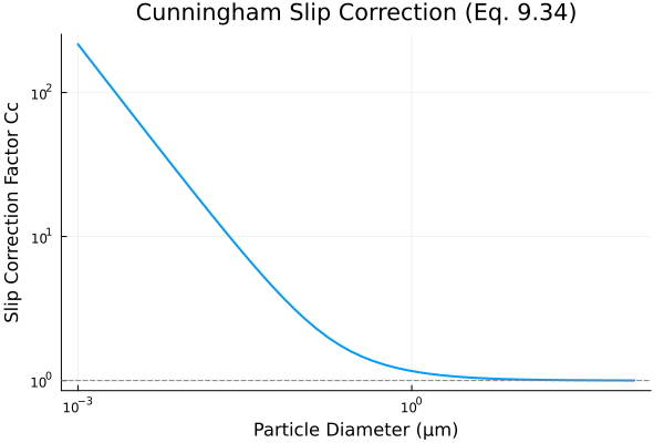
Terminal Settling Velocity vs Particle Size
The terminal settling velocity (Eq. 9.42) shows the balance between gravitational force and drag. Larger particles settle faster due to their greater mass.
v_t_values = Float64[]

for D_p in D_p_range
    prob = NonlinearProblem(csys, Dict(), Dict(csys.D_p => D_p))
    sol = solve(prob)
    push!(v_t_values, sol[csys.v_t])
end

p2 = plot(D_p_range * 1e6, v_t_values * 100 * 3600,  # Convert to cm/h
    xscale = :log10, yscale = :log10,
    xlabel = "Particle Diameter (μm)",
    ylabel = "Terminal Velocity (cm/h)",
    title = "Settling Velocity (Eq. 9.42)",
    legend = false, linewidth = 2)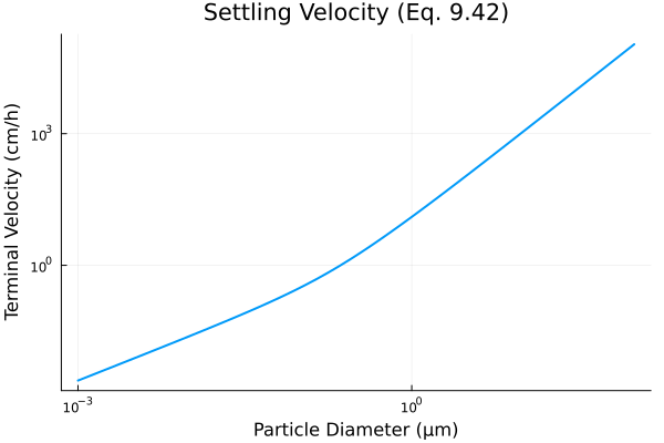
Brownian Diffusion Coefficient vs Particle Size
The Stokes-Einstein-Sutherland relation (Eq. 9.73) shows that smaller particles have larger diffusion coefficients, allowing them to spread more rapidly through random Brownian motion.
D_B_values = Float64[]

for D_p in D_p_range
    prob = NonlinearProblem(csys, Dict(), Dict(csys.D_p => D_p))
    sol = solve(prob)
    push!(D_B_values, sol[csys.D_B])
end

p3 = plot(D_p_range * 1e6, D_B_values * 1e4,  # Convert to cm²/s
    xscale = :log10, yscale = :log10,
    xlabel = "Particle Diameter (μm)",
    ylabel = "Diffusion Coefficient (cm²/s)",
    title = "Brownian Diffusivity (Eq. 9.73)",
    legend = false, linewidth = 2)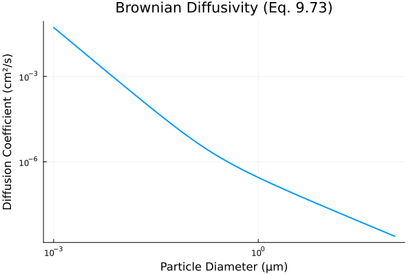
Comparison of Settling and Diffusion Timescales
The relative importance of gravitational settling versus Brownian diffusion depends on particle size. The characteristic timescale ratio τ_ds = 4D/vt² (Eq. 9.85) indicates which process dominates:
tau_ds_values = 4 .* D_B_values ./ (v_t_values .^ 2)

p4 = plot(D_p_range * 1e6, tau_ds_values,
    xscale = :log10, yscale = :log10,
    xlabel = "Particle Diameter (μm)",
    ylabel = "Characteristic Time τ_ds (s)",
    title = "Diffusion-Settling Timescale (Eq. 9.85)",
    legend = false, linewidth = 2)
hline!([1.0], linestyle = :dash, color = :gray)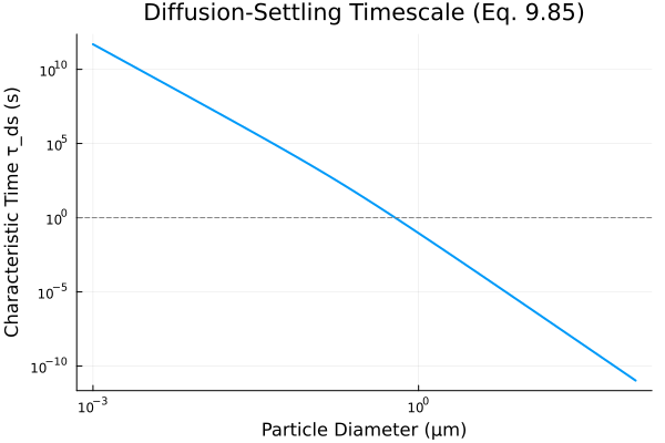
Summary Plot
plot(p1, p2, p3, p4, layout = (2, 2), size = (800, 600))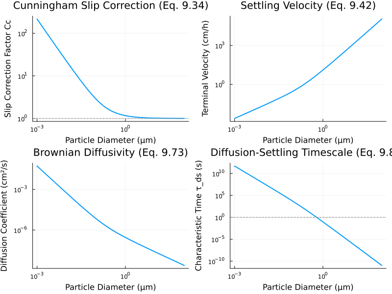
Validation Against Table 9.3: Slip Correction Factors
The following compares computed slip correction factors against values from Table 9.3 in Seinfeld & Pandis (2006):
# Reference values from Table 9.3
table_data = [
    (0.001, 216.0),
    (0.01, 22.2),
    (0.1, 2.85),
    (1.0, 1.164),
    (10.0, 1.016),
    (100.0, 1.0016)
]

D_p_table = [d[1] * 1e-6 for d in table_data]  # Convert μm to m
Cc_table = [d[2] for d in table_data]

# Computed values
Cc_computed = Float64[]
for D_p in D_p_table
    prob = NonlinearProblem(csys, Dict(), Dict(csys.D_p => D_p))
    sol = solve(prob)
    push!(Cc_computed, sol[csys.C_c])
end

DataFrame(
    Symbol("Dp (μm)") => [d[1] for d in table_data],
    Symbol("Cc (Table 9.3)") => Cc_table,
    Symbol("Cc (Computed)") => round.(Cc_computed, digits = 2),
    Symbol("Error (%)") => round.(abs.(Cc_computed .- Cc_table) ./ Cc_table .* 100, digits = 1)
)| Row | Dp (μm) | Cc (Table 9.3) | Cc (Computed) | Error (%) |
|---|---|---|---|---|
| Float64 | Float64 | Float64 | Float64 | |
| 1 | 0.001 | 216.0 | 216.39 | 0.2 |
| 2 | 0.01 | 22.2 | 22.16 | 0.2 |
| 3 | 0.1 | 2.85 | 2.86 | 0.4 |
| 4 | 1.0 | 1.164 | 1.16 | 0.0 |
| 5 | 10.0 | 1.016 | 1.02 | 0.0 |
| 6 | 100.0 | 1.0016 | 1.0 | 0.0 |
Flow Regime Classification
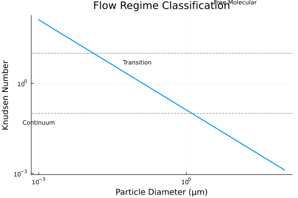
The Knudsen number determines the applicable flow regime:
| Regime | Kn Range | Description |
|---|---|---|
| Continuum | Kn → 0 | Stokes' law applies (Cc ≈ 1) |
| Transition | Kn ~ 1 | Slip correction required |
| Free molecular | Kn → ∞ | Kinetic theory applies |
plot(D_p_range * 1e6, Kn_values,
    xscale = :log10, yscale = :log10,
    xlabel = "Particle Diameter (μm)",
    ylabel = "Knudsen Number",
    title = "Flow Regime Classification",
    legend = false, linewidth = 2)
hline!([0.1, 10], linestyle = :dash, color = :gray, label = "Regime boundaries")
annotate!([(0.001, 0.05, text("Continuum", 8)),
    (0.1, 5, text("Transition", 8)),
    (10, 500, text("Free Molecular", 8))])