Cloud Physics
Overview
This module implements the cloud microphysics equations from Chapter 17 of Seinfeld & Pandis (2006), covering thermodynamic properties of water, the Kelvin (curvature) effect, Köhler theory for cloud droplet activation, diffusional growth of cloud droplets, adiabatic cooling and cloud formation dynamics, ice nucleation, rain formation, and aerosol scavenging by cloud droplets.
Reference: Seinfeld, J.H. and Pandis, S.N. (2006). Atmospheric Chemistry and Physics: From Air Pollution to Climate Change, 2nd Edition, John Wiley & Sons, Inc. Chapter 17: Cloud Physics.
Aerosol.CloudWaterProperties — Function
CloudWaterProperties(; name=:CloudWaterProperties)Thermodynamic properties of water and water solutions for cloud physics calculations, including specific heat, latent heats, surface tension, and saturation vapor pressure.
Based on Chapter 17 of Seinfeld & Pandis (2006) "Atmospheric Chemistry and Physics: From Air Pollution to Climate Change", 2nd Edition, John Wiley & Sons.
Equations 17.1-17.6, Table 17.2.
Aerosol.CloudKelvinEffect — Function
CloudKelvinEffect(; name=:CloudKelvinEffect)Kelvin (curvature) effect on vapor pressure over curved cloud droplet surfaces. The vapor pressure over a curved surface is enhanced relative to a flat surface due to surface energy effects.
Based on Equations 17.9 and 17.28 from Seinfeld & Pandis (2006) Chapter 17.
Equations
- Eq. 17.9: pw(Dp)/p° = exp(4Mw σw / (R T ρw Dp))
- Eq. 17.28: A = 4Mw σw / (R T ρ_w) ≈ 0.66/T µm (for T in K)
Aerosol.KohlerTheory — Function
KohlerTheory(; name=:KohlerTheory)Köhler theory for equilibrium vapor pressure over solution droplets, combining the Kelvin (curvature) effect and Raoult (solute) effect.
Includes standard Köhler equation, critical diameter and supersaturation, and extension for partially insoluble particles.
Based on Equations 17.26-17.40 from Seinfeld & Pandis (2006).
Key Equations
- Eq. 17.27: ln(pw(Dp)/p°) = A/Dp - B/Dp³
- Eq. 17.28: A = 4Mw σw / (R T ρ_w)
- Eq. 17.29: B = 6ns Mw / (π ρ_w)
- Eq. 17.30: D_pc = √(3B/A) (critical diameter)
- Eq. 17.32: ln(S_c) = √(4A³/27B) (critical saturation)
- Eq. 17.33: ns = νπds³ρs / (6Ms) (moles of solute)
- Eq. 17.38-17.40: Extensions for insoluble material
Aerosol.DropletGrowth — Function
DropletGrowth(; name=:DropletGrowth)Diffusional growth rate of cloud droplets by condensation of water vapor. Accounts for the thermal gradient between droplet surface and environment, gas-phase diffusion, and modified diffusivity for kinetic effects.
Based on Equations 17.60-17.72 from Seinfeld & Pandis (2006).
Key Equations
- Eq. 17.61: Dv = 0.211(pref/p)(T/273)^1.94 cm²/s (water vapor diffusivity)
- Eq. 17.62: D'v = Dv / [1 + 2Dv/(αc Dp)√(2πMw/RT)] (kinetic correction)
- Eq. 17.70: Dp dDp/dt = [Sv,∞ - Seq] / [ρw RT/(4p° D'v Mw) + ΔHv ρw/(4k'a T)(ΔHv Mw/(TR) - 1)]
- Eq. 17.71: k_a = 10⁻³(4.39 + 0.071T) J/(m·s·K) (thermal conductivity)
- Eq. 17.72: k'_a correction for kinetic effects
Aerosol.CloudDynamics — Function
CloudDynamics(; name=:CloudDynamics)Adiabatic cooling, cloud formation, and supersaturation dynamics. Includes dry adiabatic lapse rate, lifting condensation level (LCL), dew point temperature, and saturation mixing ratio.
Based on Equations 17.43-17.49 from Seinfeld & Pandis (2006).
Key Equations
- Eq. 17.43: Td ≈ T0 + (RT0²/ΔHv M_w)ln(RH) (dew point temperature)
- Eq. 17.44: Γd = g/cp ≈ 9.76 K/km (dry adiabatic lapse rate)
- Eq. 17.46: wv = Mw pw / (Ma p_a) (water vapor mixing ratio)
- Eq. 17.49: hLCL = (T0 - T_L)/Γ (lifting condensation level)
Aerosol.IcePhysics — Function
IcePhysics(; name=:IcePhysics)Ice nucleation and ice-water equilibrium thermodynamics. Includes freezing point depression for solutions, Kelvin equation for ice particles, and empirical ice nuclei concentration.
Based on Equations 17.100-17.103 from Seinfeld & Pandis (2006) "Atmospheric Chemistry and Physics: From Air Pollution to Climate Change", 2nd Edition, Chapter 17.
Key Equations
- Eq. 17.100: T0 - Te = (RT0 Te/ΔHm)(-ln aw) (freezing point from water activity)
- Eq. 17.101: ΔTf = (RT0² Mw)/(1000 ΔHm) m ≈ 1.86 K·kg/mol × m (freezing point depression)
- Eq. 17.102: pi = psat,i exp(4Mw σia / (R T ρi Dp)) (Kelvin effect for ice)
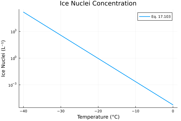
- Eq. 17.103: IN(L⁻¹) = exp[0.6(253-T)] (ice nuclei concentration)
Aerosol.RainFormation — Function
RainFormation(; name=:RainFormation)Rain formation by collision and coalescence processes, plus raindrop size distributions.
Based on Equations 17.104-17.108 from Seinfeld & Pandis (2006).
Key Equations
- Eq. 17.104: E = y²/(Dp + dp)² (collision efficiency)
- Eq. 17.105: Ec = (Dp/(Dp + dp))² (coalescence efficiency, for D_p > 400 µm)
- Eq. 17.106: dm/dt = (π/4)Et(Dp + dp)²wL(vD - vd) (continuous accretion)
- Eq. 17.107: F(Dp) = 1 - exp[-(Dp/(1.3p_0^0.232 mm))^2.25] (Best CDF)
- Eq. 17.108: n(Dp) = n0 exp(-ψD_p) (Marshall-Palmer distribution)
Aerosol.AerosolScavenging — Function
AerosolScavenging(; name=:AerosolScavenging)Aerosol scavenging by cloud droplets, including mass and number scavenging ratios and scavenging coefficients.
Based on Equations 17.84-17.92 from Seinfeld & Pandis (2006).
Key Equations
- Eq. 17.84: Fi = (C{i,0} - C{i,int})/C{i,0} (mass scavenging ratio)
- Eq. 17.85: FN = (N0 - Nint)/N0 (number scavenging ratio)
- Eq. 17.91: Λ(Dp,t) = ∫K(Dp,x)n_d(x,t)dx (scavenging coefficient)
- Eq. 17.92: Λ(Dp) = Nd K(D_p, 10µm) (monodisperse approximation)
Aerosol.CloudPhysics — Function
CloudPhysics(; name=:CloudPhysics)Complete cloud physics system composing all subsystems: water properties, Kelvin effect, Köhler theory, droplet growth, cloud dynamics, ice physics, rain formation, and aerosol scavenging.
Based on Chapter 17 of Seinfeld & Pandis (2006) "Atmospheric Chemistry and Physics: From Air Pollution to Climate Change", 2nd Edition, John Wiley & Sons.
Reference Tables
The following tables from Seinfeld & Pandis (2006) Chapter 17 provide key physical constants used in this implementation.
Table 17.1: Properties of Water
| Property | Phase/Temperature | Symbol | Value |
|---|---|---|---|
| Specific heat at constant pressure | Vapor | ĉ_pv | 1952 J kg⁻¹ K⁻¹ |
| Specific heat at constant pressure | Liquid (0°C) | ĉ_pw | 4218 J kg⁻¹ K⁻¹ |
| Specific heat at constant volume | Vapor | ĉ_vw | 1463 J kg⁻¹ K⁻¹ |
| Latent heat of evaporation | 0°C | ΔH_v | 2.5 kJ g⁻¹ |
| Latent heat of evaporation | 100°C | ΔH_v | 2.25 kJ g⁻¹ |
| Latent heat of fusion | 0°C | ΔH_m | 0.33 kJ g⁻¹ |
| Surface tension | Water/air (20°C) | σ_w0 | 0.073 J m⁻² |
Table 17.2: Saturation Vapor Pressure Polynomial Coefficients
The saturation vapor pressure over a flat surface is given by:
p°(mbar) = a₀ + a₁T + a₂T² + a₃T³ + a₄T⁴ + a₅T⁵ + a₆T⁶ (T is in °C)
| Coefficient | Water (−50 to +50°C) | Ice (−50 to 0°C) |
|---|---|---|
| a₀ | 6.107799961 | 6.109177956 |
| a₁ | 4.436518521×10⁻¹ | 5.034698970×10⁻¹ |
| a₂ | 1.428945805×10⁻² | 1.886013408×10⁻² |
| a₃ | 2.650648471×10⁻⁴ | 4.176223716×10⁻⁴ |
| a₄ | 3.031240396×10⁻⁶ | 5.824720280×10⁻⁶ |
| a₅ | 2.034080948×10⁻⁸ | 4.838803174×10⁻⁸ |
| a₆ | 6.136820929×10⁻¹¹ | 1.838826904×10⁻¹⁰ |
Source: Lowe and Ficke (1974)
Table 17.3: Updraft Velocities and Maximum Supersaturations for Clouds and Fogs
| Cloud Type | Updraft Velocity (m s⁻¹) | Maximum Supersaturation (%) | Reference |
|---|---|---|---|
| Continental cumulus | ~1–17 | 0.25–0.7 | Pruppacher and Klett (1997) |
| Maritime cumulus | ~1–2.5 | 0.3–0.8 | Pruppacher and Klett (1997); Mason (1971) |
| Stratiform | ~0–1 | ~0.05 | Pruppacher and Klett (1997) |
| Fog | — | ~0.1 | Pandis and Seinfeld (1989) |
Table 17.4: Empirical Parameters for CCN Concentration
The CCN concentration can be approximated by: CCN(s) = c·sᵏ
where CCN(s) is in particles cm⁻³ and s is supersaturation in percent.
| c (cm⁻³) | k | Location |
|---|---|---|
| 125 | 0.3 | Maritime (Australia) |
| 53–105 | 0.5–0.6 | Maui (Hawaii) |
| 100 | 0.5 | Atlantic, Pacific Oceans |
| 190 | 0.8 | Pacific |
| 250 | 1.3–1.4 | North Atlantic |
| 145–370 | 0.4–0.9 | North Atlantic |
| 100–1000 | — | Arctic |
| 140 | 0.4 | Cape Grim (Australia) |
| 250 | 0.5 | North Atlantic |
| 25–128 | 0.4–0.6 | North Pacific |
| 27–111 | 1.0 | North Pacific |
| 400 | 0.3 | Polluted North Pacific |
| 100 | 0.4 | Equatorial Pacific |
| 600 | 0.5 | Continental |
| 2000 | 0.4 | Continental (Australia) |
| 3500 | 0.9 | Continental (Buffalo, NY) |
Source: Hegg and Hobbs (1992)
Implementation
The cloud physics system is composed of eight subsystems, each implemented as a ModelingToolkit @component function. They can be used individually or composed together via the CloudPhysics parent system.
State Variables
using DataFrames, ModelingToolkit, Symbolics, DynamicQuantities
using Aerosol

sys = CloudPhysics()
vars = unknowns(sys)
DataFrame(
    :Name => [string(Symbolics.tosymbol(v, escape = false)) for v in vars],
    :Units => [string(dimension(ModelingToolkit.get_unit(v))) for v in vars],
    :Description => [ModelingToolkit.getdescription(v) for v in vars]
)| Row | Name | Units | Description |
|---|---|---|---|
| String | String | String | |
| 1 | water₊T_C | K | Temperature difference from 273.15 K |
| 2 | water₊c_pw | m² s⁻² K⁻¹ | Specific heat of liquid water |
| 3 | water₊ΔH_v | m² s⁻² | Latent heat of vaporization |
| 4 | water₊ΔH_m | m² s⁻² | Latent heat of melting |
| 5 | water₊σ_w0 | kg s⁻² | Surface tension of pure water |
| 6 | water₊p_sat_water | m⁻¹ kg s⁻² | Saturation vapor pressure over water |
| 7 | water₊p_sat_ice | m⁻¹ kg s⁻² | Saturation vapor pressure over ice |
| 8 | kelvin₊A_kelvin | m | Kelvin parameter A (Eq. 17.28) |
| 9 | kelvin₊kelvin_ratio | Kelvin ratio p_w(D_p)/p° (Eq. 17.9, dimensionless) | |
| 10 | kohler₊A | m | Kelvin parameter |
| 11 | kohler₊n_s | mol | Moles of solute |
| 12 | kohler₊B | m³ | Solute parameter |
| 13 | kohler₊d_u | m | Diameter of insoluble core |
| 14 | kohler₊ln_S | Log of saturation ratio (dimensionless) | |
| 15 | kohler₊S | Saturation ratio (dimensionless) | |
| 16 | kohler₊D_pc | m | Critical droplet diameter |
| 17 | kohler₊ln_S_c | Log of critical saturation (dimensionless) | |
| 18 | kohler₊S_c | Critical saturation ratio (dimensionless) | |
| 19 | growth₊D_v | m² s⁻¹ | Diffusivity of water vapor in air |
| 20 | growth₊D_v_prime | m² s⁻¹ | Modified diffusivity of water vapor |
| 21 | growth₊k_a | m kg s⁻³ K⁻¹ | Thermal conductivity of air |
| 22 | growth₊ρ_air | m⁻³ kg | Air density from ideal gas law (Eq. 17.72) |
| 23 | growth₊k_a_prime | m kg s⁻³ K⁻¹ | Modified thermal conductivity of air |
| 24 | growth₊p_sat | m⁻¹ kg s⁻² | Saturation vapor pressure |
| 25 | growth₊ΔH_v | m² s⁻² | Latent heat of vaporization |
| 26 | growth₊S_eq | Equilibrium saturation ratio over droplet (dimensionless) | |
| 27 | growth₊dDp_dt | m s⁻¹ | Droplet diameter growth rate |
| 28 | cloud₊Γ_d | m⁻¹ K | Dry adiabatic lapse rate |
| 29 | cloud₊p_sat | m⁻¹ kg s⁻² | Saturation vapor pressure at T_0 |
| 30 | cloud₊w_vs | Saturation mixing ratio (dimensionless) | |
| 31 | cloud₊T_d | K | Dew point temperature |
| 32 | cloud₊h_LCL | m | Lifting condensation level height |
| 33 | ice₊ΔT_f | K | Freezing point depression |
| 34 | ice₊T_e | K | Equilibrium freezing temperature |
| 35 | ice₊kelvin_ice | Kelvin factor for ice (dimensionless) | |
| 36 | ice₊IN | m⁻³ | Ice nuclei concentration |
| 37 | rain₊E_t | Collection efficiency (Eq. 17.106, dimensionless) | |
| 38 | rain₊dm_dt | kg s⁻¹ | Mass accretion rate (Eq. 17.106) |
| 39 | rain₊F_dist | Best raindrop CDF (Eq. 17.107, dimensionless) | |
| 40 | rain₊n_MP | m⁻⁴ | Marshall-Palmer number density (Eq. 17.108) |
| 41 | scav₊F_mass | Mass scavenging ratio (dimensionless) | |
| 42 | scav₊F_number | Number scavenging ratio (dimensionless) | |
| 43 | scav₊Λ | s⁻¹ | Scavenging coefficient |
Parameters
params = parameters(sys)
DataFrame(
    :Name => [string(Symbolics.tosymbol(p, escape = false)) for p in params],
    :Units => [string(dimension(ModelingToolkit.get_unit(p))) for p in params],
    :Description => [ModelingToolkit.getdescription(p) for p in params]
)| Row | Name | Units | Description |
|---|---|---|---|
| String | String | String | |
| 1 | water₊T_ref | K | Reference temperature (0°C) |
| 2 | water₊T | K | Temperature |
| 3 | water₊cpw_base | m² s⁻² K⁻¹ | Base specific heat of water (Eq. 17.2) |
| 4 | water₊T_cpw_ref | K | Reference T for c_pw correlation (Eq. 17.2) |
| 5 | water₊T_unit | K | Unit temperature for nondimensionalization |
| 6 | water₊cpw_c2 | m² s⁻² K⁻¹ | Quadratic coefficient for c_pw (Eq. 17.2: 1.3e-5 J/(g*K) * 1000) |
| 7 | water₊cpw_c4 | m² s⁻² K⁻¹ | Quartic coefficient for c_pw (Eq. 17.2: 1.6e-8 J/(g*K) * 1000) |
| 8 | water₊Hv_ref | m² s⁻² | Latent heat reference value (Eq. 17.3: 2.5 kJ/g = 2.5e6 J/kg) |
| 9 | water₊Hv_exp_const | Exponent constant for latent heat (Eq. 17.3, dimensionless) | |
| 10 | water₊Hv_exp_coeff | K⁻¹ | Exponent coefficient for latent heat (Eq. 17.3) |
| 11 | water₊Hm_base | m² s⁻² | Base latent heat of melting (Eq. 17.4: 333.5 J/g = 333500 J/kg) |
| 12 | water₊Hm_c1 | m² s⁻² | Linear coeff. for latent heat of melting (Eq. 17.4: 2.03 J/g = 2030 J/kg) |
| 13 | water₊Hm_c2 | m² s⁻² | Quadratic coeff. for latent heat of melting (Eq. 17.4: -0.0105 J/g = -10.5 J/kg) |
| 14 | water₊sigma_base | kg s⁻² | Base surface tension (Eq. 17.5) |
| 15 | water₊sigma_coeff | kg s⁻² K⁻¹ | Surface tension temperature coefficient (Eq. 17.5) |
| 16 | water₊a4_w | m⁻¹ kg s⁻² | Water sat. vap. press. coeff. a4 (Table 17.2) |
| 17 | water₊a5_w | m⁻¹ kg s⁻² | Water sat. vap. press. coeff. a5 (Table 17.2) |
| 18 | water₊a1_w | m⁻¹ kg s⁻² | Water sat. vap. press. coeff. a1 (Table 17.2) |
| 19 | water₊a0_w | m⁻¹ kg s⁻² | Water sat. vap. press. coeff. a0 (Table 17.2) |
| 20 | water₊a3_w | m⁻¹ kg s⁻² | Water sat. vap. press. coeff. a3 (Table 17.2) |
| 21 | water₊a6_w | m⁻¹ kg s⁻² | Water sat. vap. press. coeff. a6 (Table 17.2) |
| 22 | water₊a2_w | m⁻¹ kg s⁻² | Water sat. vap. press. coeff. a2 (Table 17.2) |
| 23 | water₊a6_i | m⁻¹ kg s⁻² | Ice sat. vap. press. coeff. a6 (Table 17.2) |
| 24 | water₊a5_i | m⁻¹ kg s⁻² | Ice sat. vap. press. coeff. a5 (Table 17.2) |
| 25 | water₊a1_i | m⁻¹ kg s⁻² | Ice sat. vap. press. coeff. a1 (Table 17.2) |
| 26 | water₊a2_i | m⁻¹ kg s⁻² | Ice sat. vap. press. coeff. a2 (Table 17.2) |
| 27 | water₊a0_i | m⁻¹ kg s⁻² | Ice sat. vap. press. coeff. a0 (Table 17.2) |
| 28 | water₊a3_i | m⁻¹ kg s⁻² | Ice sat. vap. press. coeff. a3 (Table 17.2) |
| 29 | water₊a4_i | m⁻¹ kg s⁻² | Ice sat. vap. press. coeff. a4 (Table 17.2) |
| 30 | kelvin₊σ_w | kg s⁻² | Surface tension of water (Table 17.1) |
| 31 | kelvin₊M_w | kg mol⁻¹ | Molecular weight of water |
| 32 | kelvin₊T | K | Temperature |
| 33 | kelvin₊R | m² kg s⁻² K⁻¹ mol⁻¹ | Universal gas constant |
| 34 | kelvin₊ρ_w | m⁻³ kg | Density of liquid water at 25°C |
| 35 | kelvin₊D_p | m | Droplet diameter |
| 36 | kohler₊σ_w | kg s⁻² | Surface tension of water |
| 37 | kohler₊M_w | kg mol⁻¹ | Molecular weight of water |
| 38 | kohler₊T | K | Temperature |
| 39 | kohler₊R | m² kg s⁻² K⁻¹ mol⁻¹ | Universal gas constant |
| 40 | kohler₊ρ_w | m⁻³ kg | Density of liquid water |
| 41 | kohler₊d_s | m | Dry particle diameter |
| 42 | kohler₊π_val | Pi (dimensionless) | |
| 43 | kohler₊ν_s | Van't Hoff factor (number of ions) (dimensionless) | |
| 44 | kohler₊ε_m | Mass fraction of soluble material (dimensionless) | |
| 45 | kohler₊M_s | kg mol⁻¹ | Molecular weight of solute |
| 46 | kohler₊ρ_u | m⁻³ kg | Density of insoluble material |
| 47 | kohler₊ρ_s | m⁻³ kg | Density of solute |
| 48 | kohler₊dim_eps | Small dimensionless value for numerical stability (dimensionless) | |
| 49 | kohler₊vol_eps | m³ | Small volume for numerical stability |
| 50 | kohler₊D_p | m | Wet droplet diameter |
| 51 | growth₊T | K | Temperature |
| 52 | growth₊T_Dv_ref | K | Reference temperature for D_v |
| 53 | growth₊p_ref | m⁻¹ kg s⁻² | Reference pressure (1 atm) |
| 54 | growth₊Dv_ref | m² s⁻¹ | Reference diffusivity at 273 K, 1 atm |
| 55 | growth₊p_a | m⁻¹ kg s⁻² | Atmospheric pressure |
| 56 | growth₊one | Unit value (dimensionless) | |
| 57 | growth₊π_val | Pi (dimensionless) | |
| 58 | growth₊M_w | kg mol⁻¹ | Molecular weight of water |
| 59 | growth₊R | m² kg s⁻² K⁻¹ mol⁻¹ | Universal gas constant |
| 60 | growth₊D_p | m | Droplet diameter |
| 61 | growth₊α_c | Mass accommodation coefficient (dimensionless) | |
| 62 | growth₊ka_c0 | m kg s⁻³ K⁻¹ | Thermal conductivity constant |
| 63 | growth₊ka_c1 | m kg s⁻³ K⁻² | Thermal conductivity slope |
| 64 | growth₊M_a | kg mol⁻¹ | Molecular weight of air |
| 65 | growth₊α_T | Thermal accommodation coefficient (dimensionless) | |
| 66 | growth₊c_p_air | m² s⁻² K⁻¹ | Specific heat of air |
| 67 | growth₊T_magnus_offset | K | Magnus temperature offset |
| 68 | growth₊magnus_a | Magnus coefficient a (dimensionless) | |
| 69 | growth₊magnus_b | K | Magnus coefficient b |
| 70 | growth₊p_sat_ref | m⁻¹ kg s⁻² | Reference saturation pressure |
| 71 | growth₊Hv_ref_kg | m² s⁻² | Reference latent heat of vaporization |
| 72 | growth₊T_Hv_ref | K | Reference temperature for latent heat |
| 73 | growth₊Hv_exp_const | Exponent constant (dimensionless) | |
| 74 | growth₊Hv_exp_coeff | K⁻¹ | Exponent coefficient |
| 75 | growth₊n_s | mol | Moles of solute in droplet |
| 76 | growth₊vol_eps | m³ | Small volume for numerical stability |
| 77 | growth₊d_u | m | Insoluble core diameter |
| 78 | growth₊ρ_w | m⁻³ kg | Density of liquid water |
| 79 | growth₊σ_w | kg s⁻² | Surface tension of water |
| 80 | growth₊S_v | Environmental saturation ratio (dimensionless) | |
| 81 | cloud₊g | m s⁻² | Gravitational acceleration |
| 82 | cloud₊c_p_air | m² s⁻² K⁻¹ | Specific heat of air at constant pressure |
| 83 | cloud₊T_magnus_offset | K | Magnus temperature offset |
| 84 | cloud₊T_0 | K | Initial temperature |
| 85 | cloud₊magnus_a | Magnus coefficient a (dimensionless) | |
| 86 | cloud₊magnus_b | K | Magnus coefficient b |
| 87 | cloud₊p_sat_ref | m⁻¹ kg s⁻² | Reference saturation pressure |
| 88 | cloud₊M_w | kg mol⁻¹ | Molecular weight of water |
| 89 | cloud₊M_a | kg mol⁻¹ | Molecular weight of air |
| 90 | cloud₊p_a | m⁻¹ kg s⁻² | Atmospheric pressure |
| 91 | cloud₊R | m² kg s⁻² K⁻¹ mol⁻¹ | Universal gas constant |
| 92 | cloud₊RH | Relative humidity (dimensionless) | |
| 93 | cloud₊ΔH_v | m² s⁻² | Latent heat of vaporization |
| 94 | ice₊K_f | kg K mol⁻¹ | Cryoscopic constant of water |
| 95 | ice₊molality | kg⁻¹ mol | Solution molality |
| 96 | ice₊T_freeze | K | Freezing point of pure water |
| 97 | ice₊R | m² kg s⁻² K⁻¹ mol⁻¹ | Universal gas constant |
| 98 | ice₊a_w | Water activity (dimensionless) | |
| 99 | ice₊dim_eps | Small dimensionless value for numerical stability (dimensionless) | |
| 100 | ice₊ΔH_m_mass | m² s⁻² | Latent heat of fusion of water |
| 101 | ice₊M_w | kg mol⁻¹ | Molecular weight of water |
| 102 | ice₊σ_ia | kg s⁻² | Ice-air surface tension |
| 103 | ice₊T | K | Temperature |
| 104 | ice₊ρ_i | m⁻³ kg | Density of ice |
| 105 | ice₊D_p | m | Ice particle diameter |
| 106 | ice₊IN_ref | m⁻³ | Ice nuclei concentration reference (per L -> per m^3) |
| 107 | ice₊IN_coeff | K⁻¹ | Ice nuclei exponential coefficient |
| 108 | ice₊T_IN_ref | K | Reference temperature for IN parameterization |
| 109 | rain₊E_coll | Collision efficiency (Eq. 17.104, dimensionless) | |
| 110 | rain₊E_coal | Coalescence efficiency (Eq. 17.105, dimensionless) | |
| 111 | rain₊D_p | m | Collector drop diameter |
| 112 | rain₊d_p | m | Collected droplet diameter |
| 113 | rain₊π_val | Pi (dimensionless) | |
| 114 | rain₊w_L | Liquid water mass mixing ratio (kg water / kg air) (dimensionless) | |
| 115 | rain₊ρ_a | m⁻³ kg | Air density |
| 116 | rain₊v_D | m s⁻¹ | Fall velocity of collector drop |
| 117 | rain₊v_d | m s⁻¹ | Fall velocity of collected droplet |
| 118 | rain₊p_0 | m s⁻¹ | Rainfall intensity (Eq. 17.107) |
| 119 | rain₊p0_unit | m s⁻¹ | Unit rainfall intensity for nondimensionalization |
| 120 | rain₊F_diam_ref | m | Best distribution diameter scale (Eq. 17.107: 1.3 mm) |
| 121 | rain₊F_exp | Best distribution exponent (Eq. 17.107, dimensionless) | |
| 122 | rain₊one | Unity (dimensionless) | |
| 123 | rain₊n_0 | m⁻⁴ | Marshall-Palmer intercept parameter (Eq. 17.108: 8000 m^-3 mm^-1) |
| 124 | rain₊ψ | m⁻¹ | Marshall-Palmer slope parameter (Eq. 17.108) |
| 125 | scav₊C_int | m⁻³ | Interstitial aerosol mass concentration |
| 126 | scav₊C_0 | m⁻³ | Initial aerosol mass concentration |
| 127 | scav₊N_int | m⁻³ | Interstitial aerosol number concentration |
| 128 | scav₊N_0 | m⁻³ | Initial aerosol number concentration |
| 129 | scav₊K_coll | m³ s⁻¹ | Collision coefficient |
| 130 | scav₊N_d | m⁻³ | Cloud droplet number concentration |
Equations
eqs = equations(sys)43-element Vector{Symbolics.Equation}:
water₊T_C(t) ~ water₊T - water₊T_ref
water₊c_pw(t) ~ water₊cpw_base + water₊cpw_c2*(((water₊T - water₊T_cpw_ref) / water₊T_unit)^2) + water₊cpw_c4*(((water₊T - water₊T_cpw_ref) / water₊T_unit)^4)
water₊ΔH_v(t) ~ ((water₊T_ref / water₊T)^(water₊Hv_exp_const + water₊Hv_exp_coeff*water₊T))*water₊Hv_ref
water₊ΔH_m(t) ~ water₊Hm_base + (water₊Hm_c1*water₊T_C(t)) / water₊T_unit + water₊Hm_c2*((water₊T_C(t) / water₊T_unit)^2)
water₊σ_w0(t) ~ water₊sigma_base - water₊T_C(t)*water₊sigma_coeff
water₊p_sat_water(t) ~ water₊a0_w + (water₊T_C(t)*water₊a1_w) / water₊T_unit + water₊a2_w*((water₊T_C(t) / water₊T_unit)^2) + water₊a3_w*((water₊T_C(t) / water₊T_unit)^3) + water₊a4_w*((water₊T_C(t) / water₊T_unit)^4) + water₊a5_w*((water₊T_C(t) / water₊T_unit)^5) + water₊a6_w*((water₊T_C(t) / water₊T_unit)^6)
water₊p_sat_ice(t) ~ water₊a0_i + (water₊T_C(t)*water₊a1_i) / water₊T_unit + water₊a2_i*((water₊T_C(t) / water₊T_unit)^2) + water₊a3_i*((water₊T_C(t) / water₊T_unit)^3) + water₊a4_i*((water₊T_C(t) / water₊T_unit)^4) + water₊a5_i*((water₊T_C(t) / water₊T_unit)^5) + water₊a6_i*((water₊T_C(t) / water₊T_unit)^6)
kelvin₊A_kelvin(t) ~ (4kelvin₊M_w*kelvin₊σ_w) / (kelvin₊R*kelvin₊T*kelvin₊ρ_w)
kelvin₊kelvin_ratio(t) ~ exp(kelvin₊A_kelvin(t) / kelvin₊D_p)
kohler₊A(t) ~ (4kohler₊M_w*kohler₊σ_w) / (kohler₊R*kohler₊T*kohler₊ρ_w)
⋮
ice₊kelvin_ice(t) ~ exp((4ice₊M_w*ice₊σ_ia) / (ice₊D_p*ice₊R*ice₊T*ice₊ρ_i))
ice₊IN(t) ~ exp(ice₊IN_coeff*(-ice₊T + ice₊T_IN_ref))*ice₊IN_ref
rain₊E_t(t) ~ rain₊E_coal*rain₊E_coll
rain₊dm_dt(t) ~ (1//4)*abs(rain₊v_D - rain₊v_d)*((rain₊D_p + rain₊d_p)^2)*rain₊E_t(t)*rain₊w_L*rain₊π_val*rain₊ρ_a
rain₊F_dist(t) ~ -exp(-((rain₊D_p / (rain₊F_diam_ref*((rain₊p_0 / rain₊p0_unit)^0.232)))^rain₊F_exp)) + rain₊one
rain₊n_MP(t) ~ exp(-rain₊D_p*rain₊ψ)*rain₊n_0
scav₊F_mass(t) ~ (scav₊C_0 - scav₊C_int) / scav₊C_0
scav₊F_number(t) ~ (scav₊N_0 - scav₊N_int) / scav₊N_0
scav₊Λ(t) ~ scav₊K_coll*scav₊N_dAnalysis
Figure 17.1: Saturation Concentration of Water Vapor vs Temperature
The saturation concentration of water vapor over a flat water surface increases approximately exponentially with temperature. This figure shows the concentration calculated from the saturation vapor pressure (Table 17.2 polynomial) using the ideal gas law: c = p·M_w / (R·T).
using Plots, NonlinearSolve

wp = CloudWaterProperties()
wp_sys = mtkcompile(wp)

M_w = 0.018015  # kg/mol, molecular weight of water
R = 8.314       # J/(mol·K), universal gas constant

T_range = 263.15:1.0:303.15  # -10°C to 30°C (matching Fig. 17.1 range)
c_sat_vals = Float64[]

for T_val in T_range
    prob = NonlinearProblem(wp_sys, Dict(wp_sys.T => T_val))
    sol = solve(prob)
    p_sat = sol[wp_sys.p_sat_water]  # Pa
    # Convert pressure to concentration: c = p·M_w / (R·T) in kg/m³, then to g/m³
    c_sat = p_sat * M_w / (R * T_val) * 1000  # g/m³
    push!(c_sat_vals, c_sat)
end

plot(T_range .- 273.15, c_sat_vals,
    xlabel = "Temperature (°C)", ylabel = "Water Vapor Concentration (g m⁻³)",
    label = "Water (Table 17.2 polynomial)",
    linewidth = 2, legend = :topleft,
    title = "Fig. 17.1: Saturation Concentration of Water Vapor")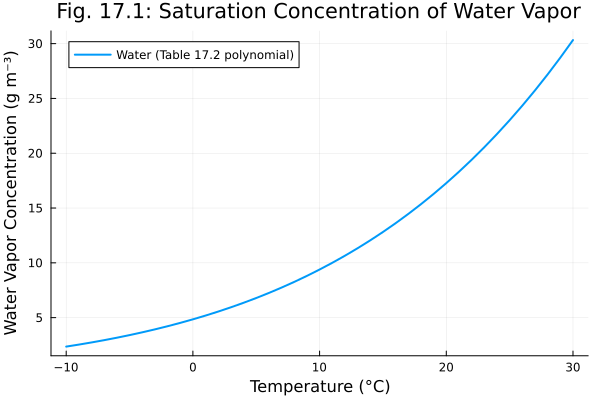
Figure 17.2: Kelvin Effect
The vapor pressure over a curved droplet surface is enhanced relative to a flat surface, with the enhancement increasing as droplet diameter decreases (Eq. 17.9).
ke = CloudKelvinEffect()
ke_sys = mtkcompile(ke)

D_p_range = 10.0 .^ range(log10(1e-8), log10(1e-5), length = 100)  # 10 nm to 10 µm
kelvin_vals = Float64[]

for D_val in D_p_range
    prob = NonlinearProblem(ke_sys, Dict(ke_sys.D_p => D_val, ke_sys.T => 293.15))
    sol = solve(prob)
    push!(kelvin_vals, sol[ke_sys.kelvin_ratio])
end

plot(D_p_range * 1e6, kelvin_vals,
    xlabel = "Droplet Diameter (µm)", ylabel = "p_w(D_p) / p°",
    xscale = :log10, label = "T = 293.15 K",
    linewidth = 2, title = "Fig. 17.2: Kelvin Effect",
    legend = :topright)
hline!([1.0], linestyle = :dash, color = :gray, label = "Flat surface")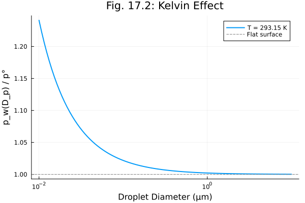
Figure 17.5: Köhler Curves
Köhler curves show the equilibrium saturation ratio as a function of wet droplet diameter for different dry particle sizes and solute compositions. The curves exhibit a maximum (critical supersaturation) beyond which droplets activate and grow without bound.
kt = KohlerTheory()
kt_sys = mtkcompile(kt)

D_wet_range = 10.0 .^ range(log10(1e-8), log10(5e-5), length = 200)

function kohler_curve(kt_sys, d_dry, M_s, rho_s, nu_s)
    S_vals = Float64[]
    for D_w in D_wet_range
        prob = NonlinearProblem(kt_sys,
            Dict(
                kt_sys.D_p => D_w, kt_sys.d_s => d_dry,
                kt_sys.M_s => M_s, kt_sys.ρ_s => rho_s,
                kt_sys.ν_s => nu_s, kt_sys.T => 293.15, kt_sys.ε_m => 1.0
            ))
        sol = solve(prob)
        push!(S_vals, sol[kt_sys.S])
    end
    return S_vals
end

# NaCl: M_s = 0.05844, rho = 2165, nu = 2
# (NH4)2SO4: M_s = 0.13214, rho = 1770, nu = 3
plot(title = "Fig. 17.5: Köhler Curves", xlabel = "Wet Diameter (µm)",
    ylabel = "Saturation Ratio S", legend = :topright, ylims = (0.990, 1.015))

for (d_dry, style) in [(0.05e-6, :solid), (0.1e-6, :dash), (0.5e-6, :dot)]
    d_label = round(d_dry * 1e6, digits = 2)
    S_nacl = kohler_curve(kt_sys, d_dry, 0.05844, 2165.0, 2.0)
    plot!(D_wet_range * 1e6, S_nacl, label = "NaCl d_s=$(d_label) µm",
        linestyle = style, linewidth = 2, color = :blue, xscale = :log10)
    S_as = kohler_curve(kt_sys, d_dry, 0.13214, 1770.0, 3.0)
    plot!(D_wet_range * 1e6, S_as, label = "(NH₄)₂SO₄ d_s=$(d_label) µm",
        linestyle = style, linewidth = 2, color = :red, xscale = :log10)
end
hline!([1.0], linestyle = :dash, color = :gray, label = "S = 1")
plot!()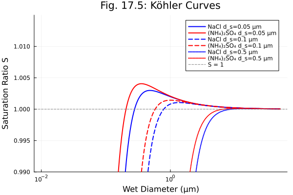
Figure 17.6: Critical Supersaturation vs Dry Diameter
Critical supersaturation decreases with increasing dry particle diameter, following a power-law relationship (Eq. 17.34).
d_dry_range = 10.0 .^ range(log10(1e-8), log10(1e-6), length = 50)

function critical_ss(kt_sys, d_dry_range, M_s, rho_s, nu_s)
    sc_vals = Float64[]
    for d_d in d_dry_range
        prob = NonlinearProblem(kt_sys,
            Dict(
                kt_sys.d_s => d_d, kt_sys.M_s => M_s, kt_sys.ρ_s => rho_s,
                kt_sys.ν_s => nu_s, kt_sys.T => 293.15, kt_sys.ε_m => 1.0
            ))
        sol = solve(prob)
        push!(sc_vals, (sol[kt_sys.S_c] - 1) * 100)  # Convert to percent
    end
    return sc_vals
end

sc_nacl = critical_ss(kt_sys, d_dry_range, 0.05844, 2165.0, 2.0)
sc_as = critical_ss(kt_sys, d_dry_range, 0.13214, 1770.0, 3.0)

plot(d_dry_range * 1e6, sc_nacl, label = "NaCl", linewidth = 2, color = :blue,
    xlabel = "Dry Diameter (µm)", ylabel = "Critical Supersaturation (%)",
    xscale = :log10, yscale = :log10, title = "Fig. 17.6: Critical Supersaturation",
    legend = :topright)
plot!(d_dry_range * 1e6, sc_as, label = "(NH₄)₂SO₄", linewidth = 2, color = :red)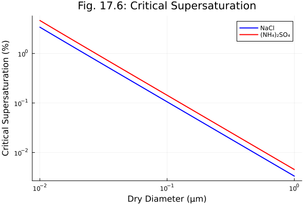
Figure 17.7: Effect of Dissociation on Köhler Curves
Köhler curves for (NH₄)₂SO₄ particles showing the effect of complete dissociation (ν=3) versus no dissociation (ν=1). Dissociation lowers the critical saturation ratio and decreases the critical diameter.
D_wet_range_17_7 = 10.0 .^ range(log10(1e-8), log10(2e-5), length = 200)

function kohler_curve_nu(kt_sys, d_dry, nu_s)
    S_vals = Float64[]
    for D_w in D_wet_range_17_7
        prob = NonlinearProblem(kt_sys,
            Dict(
                kt_sys.D_p => D_w, kt_sys.d_s => d_dry,
                kt_sys.M_s => 0.13214, kt_sys.ρ_s => 1770.0,
                kt_sys.ν_s => nu_s, kt_sys.T => 293.15, kt_sys.ε_m => 1.0
            ))
        sol = solve(prob)
        push!(S_vals, sol[kt_sys.S])
    end
    return S_vals
end

plot(title = "Fig. 17.7: Köhler Curves - Dissociation Effect",
    xlabel = "Wet Radius (µm)", ylabel = "Saturation Ratio S",
    legend = :topright, ylims = (0.998, 1.012))

for d_dry in [0.02e-6, 0.04e-6, 0.1e-6]
    d_label = round(d_dry * 1e6 * 1000, digits = 0)  # in nm
    S_complete = kohler_curve_nu(kt_sys, d_dry, 3.0)
    S_none = kohler_curve_nu(kt_sys, d_dry, 1.0)
    plot!(
        D_wet_range_17_7 * 1e6 / 2, S_complete, label = "Complete diss., r=$(d_label/2) nm",
        linestyle = :dash, linewidth = 2, xscale = :log10)
    plot!(D_wet_range_17_7 * 1e6 / 2, S_none, label = "No diss., r=$(d_label/2) nm",
        linestyle = :solid, linewidth = 2, xscale = :log10)
end
hline!([1.0], linestyle = :dot, color = :gray, label = "S = 1")
plot!()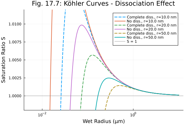
Figure 17.8: Köhler Curves with Insoluble Material
Köhler curves for particles containing (NH₄)₂SO₄ and insoluble material, showing how decreasing soluble mass fraction (ε_m) increases the supersaturation required for activation (Eqs. 17.35-17.40).
D_wet_range_17_8 = 10.0 .^ range(log10(1e-7), log10(1e-4), length = 200)

function kohler_curve_eps(kt_sys, d_dry, eps_m)
    S_vals = Float64[]
    for D_w in D_wet_range_17_8
        prob = NonlinearProblem(kt_sys,
            Dict(
                kt_sys.D_p => D_w, kt_sys.d_s => d_dry,
                kt_sys.M_s => 0.13214, kt_sys.ρ_s => 1770.0,
                kt_sys.ν_s => 3.0, kt_sys.T => 293.15, kt_sys.ε_m => eps_m,
                kt_sys.ρ_u => 2000.0
            ))
        sol = solve(prob)
        push!(S_vals, (sol[kt_sys.S] - 1) * 100)  # Convert to supersaturation %
    end
    return S_vals
end

plot(title = "Fig. 17.8: Köhler Curves with Insoluble Material",
    xlabel = "Wet Diameter (µm)", ylabel = "Supersaturation (%)",
    legend = :topright, xscale = :log10, ylims = (-0.3, 0.4))

d_dry = 0.1e-6  # 0.1 µm dry diameter
for (eps_m, color) in [(1.0, :black), (0.6, :blue), (0.4, :green), (0.2, :red)]
    S_vals = kohler_curve_eps(kt_sys, d_dry, eps_m)
    plot!(D_wet_range_17_8 * 1e6, S_vals,
        label = "ε_m = $eps_m", linewidth = 2, color = color)
end
hline!([0.0], linestyle = :dash, color = :gray, label = "S = 1 (0% SS)")
plot!()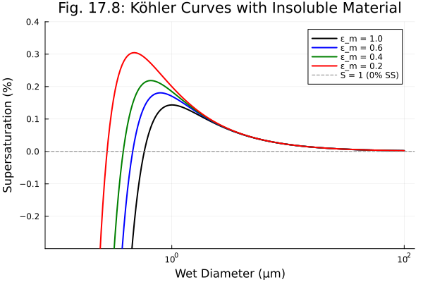
Figure 17.9: Effect of Insoluble Material on Critical Supersaturation
Particles with less soluble material require higher supersaturation to activate (Eqs. 17.35-17.40).
epsilon_vals = [1.0, 0.5, 0.1, 0.01]

plot(title = "Fig. 17.9: Insoluble Material Effect",
    xlabel = "Dry Diameter (µm)", ylabel = "Critical Supersaturation (%)",
    xscale = :log10, yscale = :log10, legend = :topright)

for eps_m in epsilon_vals
    sc_vals = Float64[]
    for d_d in d_dry_range
        prob = NonlinearProblem(kt_sys,
            Dict(
                kt_sys.d_s => d_d, kt_sys.M_s => 0.13214, kt_sys.ρ_s => 1770.0,
                kt_sys.ν_s => 3.0, kt_sys.T => 293.15, kt_sys.ε_m => eps_m,
                kt_sys.ρ_u => 2000.0
            ))
        sol = solve(prob)
        push!(sc_vals, (sol[kt_sys.S_c] - 1) * 100)
    end
    plot!(d_dry_range * 1e6, sc_vals, label = "ε_m = $eps_m", linewidth = 2)
end
plot!()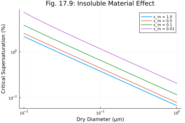
Figure 17.10: Dew Point Temperature
Dew point temperature as a function of ambient temperature for different relative humidities (Eq. 17.43).
cd = CloudDynamics()
cd_sys = mtkcompile(cd)

T0_range = 273.15:2.0:313.15  # 0°C to 40°C
RH_vals = [0.2, 0.4, 0.6, 0.8, 1.0]

plot(title = "Fig. 17.10: Dew Point Temperature",
    xlabel = "Temperature (°C)", ylabel = "Dew Point Temperature (°C)",
    legend = :bottomright)

for rh in RH_vals
    Td_vals = Float64[]
    for T0 in T0_range
        prob = NonlinearProblem(cd_sys, Dict(cd_sys.T_0 => T0, cd_sys.RH => rh))
        sol = solve(prob)
        push!(Td_vals, sol[cd_sys.T_d] - 273.15)
    end
    plot!(T0_range .- 273.15, Td_vals, label = "RH = $rh", linewidth = 2)
end
plot!()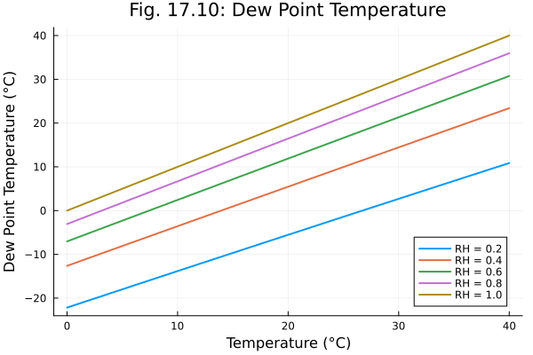
Figure 17.11: Lifting Condensation Level
Height of the lifting condensation level (LCL) as a function of surface temperature and relative humidity (Eq. 17.49).
plot(title = "Fig. 17.11: Lifting Condensation Level",
    xlabel = "Surface Temperature (°C)", ylabel = "LCL Height (m)",
    legend = :topleft)

for rh in [0.2, 0.4, 0.6, 0.8]
    h_vals = Float64[]
    for T0 in T0_range
        prob = NonlinearProblem(cd_sys, Dict(cd_sys.T_0 => T0, cd_sys.RH => rh))
        sol = solve(prob)
        push!(h_vals, sol[cd_sys.h_LCL])
    end
    plot!(T0_range .- 273.15, h_vals, label = "RH = $rh", linewidth = 2)
end
plot!()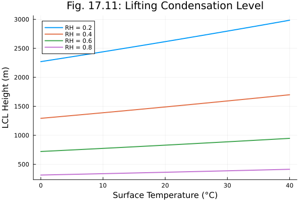
Droplet Growth Rate
Growth rate of cloud droplets as a function of diameter at 1% supersaturation (Eq. 17.70), demonstrating that smaller droplets grow faster (dDp/dt ∝ 1/Dp).
dg = DropletGrowth()
dg_sys = mtkcompile(dg)

D_range = 10.0 .^ range(log10(1e-6), log10(50e-6), length = 50)
growth_vals = Float64[]

for D_val in D_range
    prob = NonlinearProblem(dg_sys,
        Dict(
            dg_sys.D_p => D_val, dg_sys.S_v => 1.01, dg_sys.T => 293.15,
            dg_sys.n_s => 0.0, dg_sys.d_u => 0.0
        ))
    sol = solve(prob)
    push!(growth_vals, sol[dg_sys.dDp_dt])
end

plot(D_range * 1e6, growth_vals * 1e6,
    xlabel = "Droplet Diameter (µm)", ylabel = "Growth Rate dD_p/dt (µm/s)",
    linewidth = 2, label = "S = 1.01, T = 293 K",
    title = "Droplet Growth Rate (Eq. 17.70)",
    legend = :topright)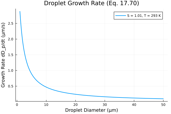
Ice Nuclei Concentration
Ice nuclei concentration increases exponentially with decreasing temperature (Eq. 17.103).
ice = IcePhysics()
ice_sys = mtkcompile(ice)

T_ice_range = 233.15:1.0:273.15  # -40°C to 0°C
IN_vals = Float64[]

for T_val in T_ice_range
    prob = NonlinearProblem(ice_sys, Dict(ice_sys.T => T_val, ice_sys.a_w => 1.0))
    sol = solve(prob)
    push!(IN_vals, sol[ice_sys.IN] / 1000.0)  # Convert from /m³ to /L
end

plot(T_ice_range .- 273.15, IN_vals,
    xlabel = "Temperature (°C)", ylabel = "Ice Nuclei (L⁻¹)",
    yscale = :log10, linewidth = 2, label = "Eq. 17.103",
    title = "Ice Nuclei Concentration",
    legend = :topright)