Organic Atmospheric Aerosols
Overview
This module implements key equations from Chapter 14 of Seinfeld and Pandis (2006) for organic atmospheric aerosol modeling, including:
- The EC tracer method for estimating secondary organic carbon
- Gas-particle partitioning models for SOA formation (noninteracting, absorptive, two-product)
- Adsorption isotherms (Langmuir, BET, FHH)
Reference: Seinfeld, J. H. and Pandis, S. N. (2006). Atmospheric Chemistry and Physics: From Air Pollution to Climate Change, 2nd Edition, Chapter 14. John Wiley & Sons, Inc.
Aerosol.ECTracerMethod — Function
ECTracerMethod(; name=:ECTracerMethod)The elemental carbon (EC) tracer method for estimating secondary organic carbon (OC) concentrations from measurements of total OC and EC.
From Seinfeld and Pandis (2006), Chapter 14, Section 14.3.2, Equations 14.1-14.4.
Primary OC is estimated as the sum of combustion-related OC (proportional to EC via the OC_EC_ratio) and noncombustion OC (OC_NC). Secondary OC is the remainder.
Reference: Seinfeld, J. H. and Pandis, S. N. (2006). Atmospheric Chemistry and Physics: From Air Pollution to Climate Change, 2nd Edition, Chapter 14. John Wiley & Sons, Inc.
Aerosol.NoninteractingSOA — Function
NoninteractingSOA(; name=:NoninteractingSOA)Gas-particle partitioning model for a secondary organic aerosol (SOA) compound that does not interact with preexisting aerosol components. The compound exists in the aerosol phase as pure compound, so gas-aerosol equilibrium is reached when the gas-phase concentration equals the saturation concentration.
From Seinfeld and Pandis (2006), Chapter 14, Section 14.5.2, Equations 14.6-14.18.
The aerosol concentration is zero until the reacted ROG exceeds the threshold ΔROG*_i = p°_i M_ROG / (a_i R T), after which the excess condenses.
Reference: Seinfeld, J. H. and Pandis, S. N. (2006). Atmospheric Chemistry and Physics: From Air Pollution to Climate Change, 2nd Edition, Chapter 14. John Wiley & Sons, Inc.
Aerosol.AbsorptivePartitioning — Function
AbsorptivePartitioning(; name=:AbsorptivePartitioning)Gas-particle partitioning model for SOA formation by absorption into a preexisting organic aerosol phase, assuming an ideal solution. There is no threshold for SOA formation; secondary aerosol forms as soon as the ROG starts reacting.
From Seinfeld and Pandis (2006), Chapter 14, Section 14.5.2, Equations 14.19-14.26.
Uses the dilute approximation c_{aer,i} << m_0 (Eq. 14.23), valid when no single compound dominates the organic aerosol composition.
Reference: Seinfeld, J. H. and Pandis, S. N. (2006). Atmospheric Chemistry and Physics: From Air Pollution to Climate Change, 2nd Edition, Chapter 14. John Wiley & Sons, Inc.
Aerosol.TwoProductSOA — Function
TwoProductSOA(; name=:TwoProductSOA)The two-product model for secondary organic aerosol (SOA) formation, developed by Odum et al. (1996). This model represents the complex mixture of oxidation products from a reactive organic gas (ROG) as two lumped surrogate products that form an ideal solution.
From Seinfeld and Pandis (2006), Chapter 14, Section 14.5.2, Equations 14.27-14.43.
The key equation (14.43) gives the overall aerosol mass yield:
Y = c_aer * (a₁/(c_aer + c₁°) + a₂/(c_aer + c₂°))where a_i are stoichiometric yields and c_i° are saturation concentrations.
Parameters from Table 14.12 are provided for multiple VOC precursors.
Reference: Seinfeld, J. H. and Pandis, S. N. (2006). Atmospheric Chemistry and Physics: From Air Pollution to Climate Change, 2nd Edition, Chapter 14. John Wiley & Sons, Inc.
See also: Odum, J. R. et al. (1996). Gas/Particle Partitioning and Secondary Organic Aerosol Yields. Environ. Sci. Technol., 30, 2580-2585.
Aerosol.LangmuirAdsorption — Function
LangmuirAdsorption(; name=:LangmuirAdsorption)Langmuir adsorption isotherm for the formation of a monolayer of adsorbed molecules on particle surfaces. Assumes all adsorption sites are equivalent, no horizontal interactions, and uniform heat of adsorption.
From Seinfeld and Pandis (2006), Chapter 14, Section 14.5.3, Equation 14.44.
Reference: Seinfeld, J. H. and Pandis, S. N. (2006). Atmospheric Chemistry and Physics: From Air Pollution to Climate Change, 2nd Edition, Chapter 14. John Wiley & Sons, Inc.
Aerosol.BETAdsorption — Function
BETAdsorption(; name=:BETAdsorption)BET (Brunauer-Emmett-Teller) adsorption isotherm for multilayer adsorption. Extends the Langmuir model to include formation of additional molecular layers, assuming each adsorbed molecule can serve as an adsorption site for the next layer.
From Seinfeld and Pandis (2006), Chapter 14, Section 14.5.3, Equation 14.45.
Reference: Seinfeld, J. H. and Pandis, S. N. (2006). Atmospheric Chemistry and Physics: From Air Pollution to Climate Change, 2nd Edition, Chapter 14. John Wiley & Sons, Inc.
Aerosol.FHHAdsorption — Function
FHHAdsorption(; name=:FHHAdsorption)FHH (Frenkel-Halsey-Hill) adsorption isotherm, appropriate for conditions near saturation where the BET theory breaks down. Relates the logarithm of the supersaturation ratio to the adsorbed volume.
From Seinfeld and Pandis (2006), Chapter 14, Section 14.5.3, Equation 14.46.
Reference: Seinfeld, J. H. and Pandis, S. N. (2006). Atmospheric Chemistry and Physics: From Air Pollution to Climate Change, 2nd Edition, Chapter 14. John Wiley & Sons, Inc.
Implementation
EC Tracer Method (Section 14.3.2)
The EC tracer method estimates secondary organic carbon from measurements of total OC and EC.
using Aerosol
using ModelingToolkit
using DataFrames, Symbolics, DynamicQuantities

sys = ECTracerMethod()
vars = unknowns(sys)
DataFrame(
    :Name => [string(Symbolics.tosymbol(v, escape = false)) for v in vars],
    :Units => [string(dimension(ModelingToolkit.get_unit(v))) for v in vars],
    :Description => [ModelingToolkit.getdescription(v) for v in vars]
)| Row | Name | Units | Description |
|---|---|---|---|
| String | String | String | |
| 1 | OC_primary | m⁻³ kg | Primary organic carbon concentration |
| 2 | EC | m⁻³ kg | Elemental carbon concentration |
| 3 | OC_secondary | m⁻³ kg | Secondary organic carbon concentration |
| 4 | OC | m⁻³ kg | Total organic carbon concentration |
equations(sys)2-element Vector{Symbolics.Equation}:
OC_primary(t) ~ OC_NC + EC(t)*OC_EC_ratio
OC_secondary(t) ~ max(zero_conc, OC(t) - OC_primary(t))Noninteracting SOA (Section 14.5.2)
Gas-particle partitioning for a compound that condenses as a pure phase.
sys_ni = NoninteractingSOA()
vars = unknowns(sys_ni)
DataFrame(
    :Name => [string(Symbolics.tosymbol(v, escape = false)) for v in vars],
    :Units => [string(dimension(ModelingToolkit.get_unit(v))) for v in vars],
    :Description => [ModelingToolkit.getdescription(v) for v in vars]
)| Row | Name | Units | Description |
|---|---|---|---|
| String | String | String | |
| 1 | c_eq | m⁻³ kg | Equilibrium gas-phase saturation concentration |
| 2 | c_total | m⁻³ kg | Total product concentration |
| 3 | ΔROG | m⁻³ kg | Reacted ROG concentration |
| 4 | ΔROG_threshold | m⁻³ kg | Threshold reacted ROG for SOA formation |
| 5 | c_aer | m⁻³ kg | Aerosol-phase concentration of product |
| 6 | c_gas | m⁻³ kg | Gas-phase concentration of product |
| 7 | X_p | Mass fraction of product in aerosol phase (dimensionless) | |
| 8 | Y | Aerosol mass yield (dimensionless) |
equations(sys_ni)7-element Vector{Symbolics.Equation}:
c_eq(t) ~ (M_i*p_i) / (R_gas*T)
c_total(t) ~ (M_i*a_i*ΔROG(t)) / M_ROG
ΔROG_threshold(t) ~ (M_ROG*p_i) / (R_gas*T*a_i)
c_aer(t) ~ max(zero_conc, -c_eq(t) + c_total(t))
c_gas(t) ~ -c_aer(t) + c_total(t)
X_p(t) ~ ifelse(zero_conc < c_total(t), c_aer(t) / c_total(t), zero_dimless)
Y(t) ~ ifelse(zero_conc < ΔROG(t), c_aer(t) / ΔROG(t), zero_dimless)Absorptive Partitioning (Section 14.5.2)
SOA formation by absorption into a preexisting organic aerosol phase.
sys_ap = AbsorptivePartitioning()
vars = unknowns(sys_ap)
DataFrame(
    :Name => [string(Symbolics.tosymbol(v, escape = false)) for v in vars],
    :Units => [string(dimension(ModelingToolkit.get_unit(v))) for v in vars],
    :Description => [ModelingToolkit.getdescription(v) for v in vars]
)| Row | Name | Units | Description |
|---|---|---|---|
| String | String | String | |
| 1 | c_aer | m⁻³ kg | Aerosol-phase concentration of product i |
| 2 | ΔROG | m⁻³ kg | Reacted ROG concentration |
| 3 | X_p | Mass fraction of product in aerosol phase (dimensionless) | |
| 4 | Y | Aerosol mass yield (dimensionless) |
equations(sys_ap)3-element Vector{Symbolics.Equation}:
c_aer(t) ~ (M_i*R_gas*T*a_i*m_0*ΔROG(t)) / (M_ROG*(M_0*p_i + R_gas*T*m_0))
X_p(t) ~ (R_gas*T*m_0) / (M_0*p_i + R_gas*T*m_0)
Y(t) ~ ifelse(zero_conc < ΔROG(t), c_aer(t) / ΔROG(t), zero_dimless)Two-Product SOA Model (Section 14.5.2)
The Odum et al. (1996) two-product model for SOA formation.
sys_tp = TwoProductSOA()
vars = unknowns(sys_tp)
DataFrame(
    :Name => [string(Symbolics.tosymbol(v, escape = false)) for v in vars],
    :Units => [string(dimension(ModelingToolkit.get_unit(v))) for v in vars],
    :Description => [ModelingToolkit.getdescription(v) for v in vars]
)| Row | Name | Units | Description |
|---|---|---|---|
| String | String | String | |
| 1 | Y | Aerosol mass yield (dimensionless) | |
| 2 | c_aer | m⁻³ kg | Total organic aerosol concentration produced |
| 3 | ΔROG_threshold | m⁻³ kg | Threshold reacted ROG for binary solution SOA formation |
| 4 | ΔROG | m⁻³ kg | Reacted ROG concentration |
equations(sys_tp)3-element Vector{Symbolics.Equation}:
Y(t) ~ c_aer(t)*(a_1 / (c_aer(t) + c_sat_1) + a_2 / (c_aer(t) + c_sat_2))
ΔROG_threshold(t) ~ 1 / (a_1 / c_sat_1 + a_2 / c_sat_2)
c_aer(t) ~ Y(t)*ΔROG(t)Table 14.12: Two-Product SOA Model Parameters
Parameters for the two-product model from Seinfeld and Pandis (2006), Table 14.12. Default values correspond to α-pinene/OH oxidation.
| Parent ROG | Oxidant | α₁ | α₂ | c₁° (μg/m³) | c₂° (μg/m³) |
|---|---|---|---|---|---|
| Toluene | OH | 0.071 | 0.138 | 18.9 | 526 |
| Xylenes | OH | 0.038 | 0.167 | 23.8 | 714 |
| α-pinene | OH | 0.038 | 0.326 | 5.8 | 250 |
| α-pinene | O₃ | 0.125 | 0.102 | 11.4 | 12.7 |
| β-pinene | OH | 0.13 | 0.041 | 22.7 | 204 |
| β-pinene | O₃ | 0.21 | 0.49 | 5.1 | 333 |
| Δ³-carene | OH | 0.054 | 0.517 | 23.2 | 238 |
| Δ³-carene | O₃ | 0.128 | 0.068 | 7.8 | 14.7 |
| Δ³-carene | NO₃ | 0.743 | 0.257 | 113 | 120 |
| Caryophyllene | OH | 1.0 | - | 23 | - |
| Humulene | OH | 1.0 | - | 20 | - |
Note: Molar stoichiometric yields (α) are derived assuming that the precursor and the SOA species have the same molecular weight. Saturation mixing ratios (c°) are based on experiments at around 310 K. Source: Griffin et al. (1999).
The saturation concentrations c₁° and c₂° in the table are in μg/m³. The implementation uses SI units (kg/m³), so multiply by 10⁻⁹ when setting parameters.
Adsorption Isotherms (Section 14.5.3)
sys_lang = LangmuirAdsorption()
equations(sys_lang)
1-element Vector{Symbolics.Equation}:
V(t) ~ (V_m*b*p(t)) / (1 + b*p(t))sys_bet = BETAdsorption()
equations(sys_bet)1-element Vector{Symbolics.Equation}:
V(t) ~ (S(t)*V_m*c_BET) / ((1 - S(t))*(1 + S(t)*(-1 + c_BET)))sys_fhh = FHHAdsorption()
equations(sys_fhh)1-element Vector{Symbolics.Equation}:
V(t) ~ V_m*((A_FHH / log(1 / S(t)))^(1 / B_FHH))Analysis
Noninteracting SOA: Aerosol Yield vs Reacted ROG
This figure demonstrates the threshold behavior of noninteracting SOA formation. Below the threshold ΔROG, all product remains in the gas phase. Above it, the aerosol yield increases with increasing reacted ROG.
using NonlinearSolve, Plots

sys_ni = NoninteractingSOA()
sys_ni_nns = ModelingToolkit.toggle_namespacing(sys_ni, false)
ssys_ni = mtkcompile(sys_ni; inputs = [sys_ni_nns.ΔROG])

# Compute threshold from default parameters
R = 8.314;
T = 298.0;
p_i = 1.01325e-5;
M_i = 0.180;
M_ROG = 0.150;
a_i = 0.05
threshold = p_i * M_ROG / (a_i * R * T)

# Sweep ΔROG from 0 to 20× threshold
ΔROG_vals = range(0, 20 * threshold, length = 200)
Y_vals = Float64[]
for drog in ΔROG_vals
    prob = NonlinearProblem(ssys_ni,
        Dict(
            ssys_ni.ΔROG => drog,
            ssys_ni.c_eq => 1e-10, ssys_ni.c_total => 1e-10,
            ssys_ni.c_aer => 1e-10, ssys_ni.c_gas => 1e-10,
            ssys_ni.ΔROG_threshold => 1e-10,
            ssys_ni.X_p => 0.5, ssys_ni.Y => 0.01))
    sol = solve(prob)
    push!(Y_vals, sol[ssys_ni.Y])
end

plot(ΔROG_vals ./ threshold, Y_vals,
    xlabel = "ΔROG / ΔROG*", ylabel = "Aerosol Mass Yield Y",
    title = "Noninteracting SOA: Yield vs Reacted ROG",
    label = "Y (Eq. 14.16)", legend = :bottomright, lw = 2)
vline!([1.0], label = "Threshold ΔROG*", ls = :dash, color = :red)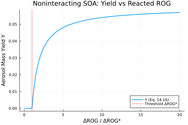
Absorptive Partitioning: Effect of Preexisting OA
When preexisting organic aerosol is present, there is no threshold for SOA formation. The aerosol mass fraction X_p depends on the ratio of absorbing medium concentration to vapor pressure.
sys_ap = AbsorptivePartitioning()
sys_ap_nns = ModelingToolkit.toggle_namespacing(sys_ap, false)
ssys_ap = mtkcompile(sys_ap; inputs = [sys_ap_nns.ΔROG])

# Sweep m_0 (preexisting OA) from 0.1 to 100 μg/m³
m0_vals = 10 .^ range(-10, -7, length = 100)  # kg/m³
Xp_vals = Float64[]
for m0 in m0_vals
    prob = NonlinearProblem(ssys_ap,
        Dict(
            ssys_ap.ΔROG => 50e-9,
            ssys_ap.c_aer => 1e-10, ssys_ap.X_p => 0.5, ssys_ap.Y => 0.01,
            ssys_ap.m_0 => m0))
    sol = solve(prob)
    push!(Xp_vals, sol[ssys_ap.X_p])
end

plot(m0_vals * 1e9, Xp_vals,
    xlabel = "Preexisting OA m₀ (μg/m³)", ylabel = "Mass Fraction in Aerosol X_p",
    title = "Absorptive Partitioning: X_p vs m₀ (Eq. 14.25)",
    label = "X_p", xscale = :log10, lw = 2, legend = :bottomright)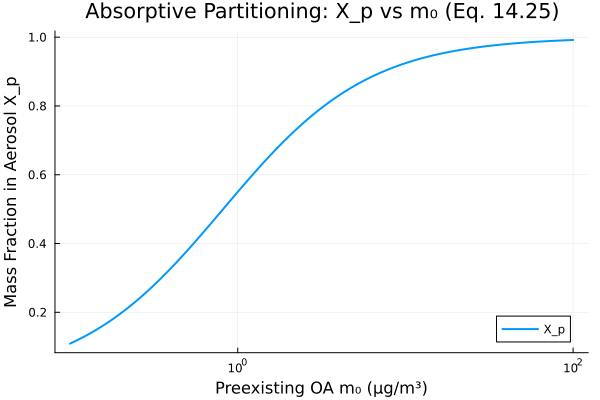
Two-Product Model: Odum Yield Curve
The two-product model (Odum et al., 1996) shows that aerosol yield increases with increasing organic aerosol concentration. This nonlinear behavior is captured by Equation 14.43.
sys_tp = TwoProductSOA()
sys_tp_nns = ModelingToolkit.toggle_namespacing(sys_tp, false)
ssys_tp = mtkcompile(sys_tp; inputs = [sys_tp_nns.ΔROG])

# Default α-pinene/OH parameters
a_1 = 0.038;
a_2 = 0.326
c_sat_1 = 5.8e-9;
c_sat_2 = 250.0e-9  # kg/m³

# Sweep ΔROG and plot Y vs c_aer (Odum plot)
ΔROG_vals = 10 .^ range(-10, -6, length = 100)  # kg/m³
c_aer_vals = Float64[]
Y_vals = Float64[]

for drog in ΔROG_vals
    prob = NonlinearProblem(ssys_tp,
        Dict(
            ssys_tp.ΔROG => drog,
            ssys_tp.c_aer => drog * 0.1,
            ssys_tp.Y => 0.1, ssys_tp.ΔROG_threshold => 1e-9))
    sol = solve(prob)
    push!(c_aer_vals, sol[ssys_tp.c_aer])
    push!(Y_vals, sol[ssys_tp.Y])
end

plot(c_aer_vals * 1e9, Y_vals,
    xlabel = "Organic Aerosol m₀ (μg/m³)", ylabel = "Aerosol Yield Y",
    title = "Two-Product Model: Yield vs Organic Aerosol (Eq. 14.43)",
    label = "α-pinene/OH", xscale = :log10, lw = 2, legend = :bottomright)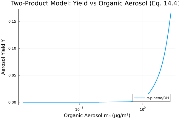
Langmuir Adsorption Isotherm
The Langmuir isotherm shows saturation behavior at high pressures.
sys_lang = LangmuirAdsorption()
sys_lang_nns = ModelingToolkit.toggle_namespacing(sys_lang, false)
ssys_lang = mtkcompile(sys_lang; inputs = [sys_lang_nns.p])

p_vals = 10 .^ range(-3, 3, length = 200)
V_vals = Float64[]
for pv in p_vals
    prob = NonlinearProblem(ssys_lang, Dict(ssys_lang.p => pv, ssys_lang.V => 0.5))
    sol = solve(prob)
    push!(V_vals, sol[ssys_lang.V])
end

plot(p_vals, V_vals,
    xlabel = "Pressure p (Pa)", ylabel = "Adsorbed Volume V (m³)",
    title = "Langmuir Adsorption Isotherm (Eq. 14.44)",
    label = "V/V_m", xscale = :log10, lw = 2, legend = :bottomright)
hline!([1.0], label = "V_m (monolayer)", ls = :dash, color = :red)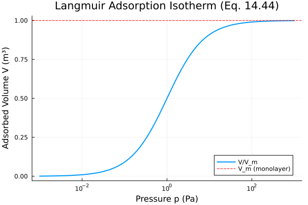
Comparison of BET and Langmuir Isotherms
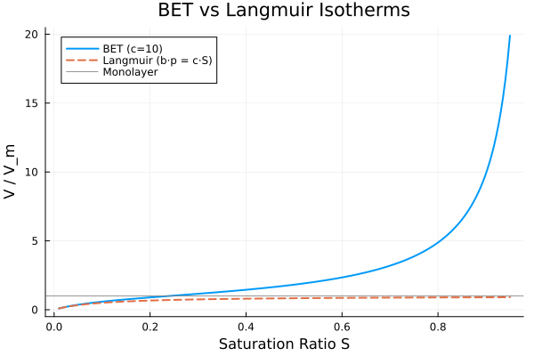
The BET isotherm extends the Langmuir model to multilayer adsorption. At low saturation ratios, both isotherms agree; at higher values, BET predicts additional adsorption layers.
sys_bet = BETAdsorption()
sys_bet_nns = ModelingToolkit.toggle_namespacing(sys_bet, false)
ssys_bet = mtkcompile(sys_bet; inputs = [sys_bet_nns.S])

S_vals = range(0.01, 0.95, length = 200)
V_bet = Float64[]
V_lang = Float64[]
c_BET = 10.0

for sv in S_vals
    # BET
    prob_bet = NonlinearProblem(ssys_bet, Dict(ssys_bet.S => sv, ssys_bet.V => 1.0))
    sol_bet = solve(prob_bet)
    push!(V_bet, sol_bet[ssys_bet.V])

    # Equivalent Langmuir: b*p = c_BET*S
    prob_lang = NonlinearProblem(ssys_lang, Dict(ssys_lang.p => c_BET * sv, ssys_lang.V => 0.5))
    sol_lang = solve(prob_lang)
    push!(V_lang, sol_lang[ssys_lang.V])
end

plot(S_vals, V_bet, label = "BET (c=10)", lw = 2,
    xlabel = "Saturation Ratio S", ylabel = "V / V_m",
    title = "BET vs Langmuir Isotherms")
plot!(S_vals, V_lang, label = "Langmuir (b·p = c·S)", lw = 2, ls = :dash)
hline!([1.0], label = "Monolayer", ls = :dot, color = :gray)