Interaction of Aerosols with Radiation
Overview
This module implements the theory of light scattering, absorption, and extinction by spherical aerosol particles, based on Mie theory and its limiting cases. These optical properties are fundamental to understanding visibility, radiative transfer, and the direct radiative forcing of aerosols.
Reference: Seinfeld, J. H., & Pandis, S. N. (2006). Atmospheric Chemistry and Physics: From Air Pollution to Climate Change (2nd ed.), Chapter 15: Interaction of Aerosols with Radiation.
Aerosol.MieScattering — Function
MieScattering(; name=:MieScattering)Mie theory for scattering and absorption of light by spherical particles.
This implements the equations from Chapter 15 of Seinfeld & Pandis (2006) "Atmospheric Chemistry and Physics: From Air Pollution to Climate Change".
The Mie theory calculates the scattering and extinction efficiencies (Qscat, Qext) as functions of the size parameter α = πDₚ/λ and the complex refractive index m = n + ik.
Key Variables
Q_scat: Scattering efficiency (dimensionless)Q_abs: Absorption efficiency (dimensionless)Q_ext: Extinction efficiency (dimensionless)ω: Single-scattering albedo (dimensionless)C_scat,C_abs,C_ext: Cross sections (m²)E_scat,E_abs,E_ext: Mass efficiencies (m²/kg)
Key Parameters
D_p: Particle diameter (m)λ: Wavelength of incident radiation (m)n_refr: Real part of refractive index (dimensionless)k_refr: Imaginary part of refractive index (dimensionless)ρ_p: Particle density (kg/m³)
Reference
Seinfeld, J. H., & Pandis, S. N. (2006). Atmospheric Chemistry and Physics (2nd ed.), Chapter 15, Equations 15.1-15.23, 15.37-15.43.
Aerosol.RayleighScattering — Function
RayleighScattering(; name=:RayleighScattering)Rayleigh scattering regime for particles much smaller than the wavelength (α << 1).
This provides closed-form solutions valid when Dp << λ (typically Dp ≤ 0.1 μm for visible light). In this regime:
- Scattered intensity is proportional to 1/λ⁴
- Scattering pattern is symmetric in forward/backward directions
- Absorption dominates over scattering (Qabs >> Qscat)
Reference
Seinfeld & Pandis (2006), Chapter 15, Equations 15.17-15.21.
Aerosol.AerosolExtinction — Function
AerosolExtinction(; name=:AerosolExtinction)Extinction coefficient calculation for an aerosol population.
Computes the extinction, scattering, and absorption coefficients (bext, bscat, b_abs) for an ensemble of particles. For a monodisperse population, these are related to the single-particle cross sections by multiplication with the number concentration.
Reference
Seinfeld & Pandis (2006), Chapter 15, Equations 15.24-15.30, 15.37-15.40.
Aerosol.Visibility — Function
Visibility(; name=:Visibility)Visibility calculation from extinction coefficient.
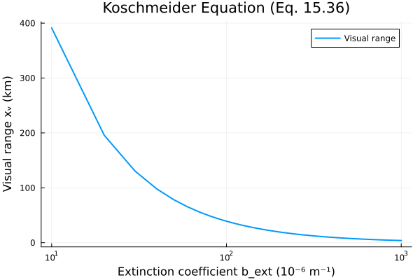
Computes visual range using the Koschmeider equation (Eq. 15.36) and related visibility metrics. Visual range is the distance at which a black object against a white background reaches the threshold contrast of 0.02.
Reference
Seinfeld & Pandis (2006), Chapter 15, Equations 15.31-15.36.
Aerosol.RayleighAtmosphere — Function
RayleighAtmosphere(; name=:RayleighAtmosphere)Calculate the Rayleigh scattering coefficient for air molecules.
The Rayleigh scattering coefficient represents the irreducible minimum of light scattering along an atmospheric sight path due to air molecules. It varies with temperature, pressure, and wavelength according to λ⁻⁴.
At sea level (T = 293 K, p = 1 atm) and λ = 550 nm, b_sg ≈ 13.2 × 10⁻⁶ m⁻¹, limiting visibility in a clean atmosphere to approximately 296 km.
Reference
Seinfeld & Pandis (2006), Chapter 15, page 705 and Problem 15.1A.
Implementation
MieScattering Component
The MieScattering component computes single-particle optical properties using full Mie theory. The key equations are:
- Size parameter (Eq. 15.6): $\alpha = \pi D_p / \lambda$
- Extinction efficiency (Eq. 15.14): $Q_{\text{ext}} = \frac{2}{\alpha^2} \sum_{k=1}^{\infty} (2k+1) \text{Re}(a_k + b_k)$
- Scattering efficiency (Eq. 15.13): $Q_{\text{scat}} = \frac{2}{\alpha^2} \sum_{k=1}^{\infty} (2k+1)(|a_k|^2 + |b_k|^2)$
- Absorption efficiency (Eq. 15.4): $Q_{\text{abs}} = Q_{\text{ext}} - Q_{\text{scat}}$
- Single-scattering albedo (Eq. 15.5): $\omega = Q_{\text{scat}} / Q_{\text{ext}}$
- Mass extinction efficiency (Eq. 15.41): $E_{\text{ext}} = \frac{3 Q_{\text{ext}}}{2 \rho_p D_p}$
where $a_k$ and $b_k$ are the Mie coefficients computed using the Bohren & Huffman (1983) algorithm.
State Variables
using DataFrames, ModelingToolkit, Symbolics, DynamicQuantities
using Aerosol

sys = MieScattering()
vars = unknowns(sys)
DataFrame(
    :Name => [string(Symbolics.tosymbol(v, escape = false)) for v in vars],
    :Units => [dimension(ModelingToolkit.get_unit(v)) for v in vars],
    :Description => [ModelingToolkit.getdescription(v) for v in vars]
)| Row | Name | Units | Description |
|---|---|---|---|
| String | Dimensio… | String | |
| 1 | α | Size parameter (dimensionless) | |
| 2 | Q_ext | Extinction efficiency (dimensionless) | |
| 3 | Q_scat | Scattering efficiency (dimensionless) | |
| 4 | Q_abs | Absorption efficiency (dimensionless) | |
| 5 | ω | Single-scattering albedo (dimensionless) | |
| 6 | C_scat | m² | Scattering cross section |
| 7 | C_abs | m² | Absorption cross section |
| 8 | C_ext | m² | Extinction cross section |
| 9 | E_ext | m² kg⁻¹ | Mass extinction efficiency |
| 10 | E_scat | m² kg⁻¹ | Mass scattering efficiency |
| 11 | E_abs | m² kg⁻¹ | Mass absorption efficiency |
Parameters
ps = parameters(sys)
DataFrame(
    :Name => [string(Symbolics.tosymbol(p, escape = false)) for p in ps],
    :Units => [dimension(ModelingToolkit.get_unit(p)) for p in ps],
    :Description => [ModelingToolkit.getdescription(p) for p in ps]
)| Row | Name | Units | Description |
|---|---|---|---|
| String | Dimensio… | String | |
| 1 | π_val | Pi (dimensionless) | |
| 2 | D_p | m | Particle diameter |
| 3 | λ | m | Wavelength of incident radiation |
| 4 | n_refr | Real part of complex refractive index (dimensionless) | |
| 5 | k_refr | Imaginary part of complex refractive index (dimensionless) | |
| 6 | ρ_p | m⁻³ kg | Particle density |
Equations
equations(sys)11-element Vector{Symbolics.Equation}:
α(t) ~ (D_p*π_val) / λ
Q_ext(t) ~ Aerosol.mie_Q_ext(α(t), n_refr, k_refr)
Q_scat(t) ~ Aerosol.mie_Q_scat(α(t), n_refr, k_refr)
Q_abs(t) ~ Q_ext(t) - Q_scat(t)
ω(t) ~ Q_scat(t) / Q_ext(t)
C_scat(t) ~ (1//4)*(D_p^2)*Q_scat(t)*π_val
C_abs(t) ~ (1//4)*(D_p^2)*Q_abs(t)*π_val
C_ext(t) ~ (1//4)*(D_p^2)*Q_ext(t)*π_val
E_ext(t) ~ (3Q_ext(t)) / (2D_p*ρ_p)
E_scat(t) ~ (3Q_scat(t)) / (2D_p*ρ_p)
E_abs(t) ~ (3Q_abs(t)) / (2D_p*ρ_p)RayleighScattering Component
The RayleighScattering component provides the closed-form Rayleigh approximation valid when $\alpha \ll 1$ (particles much smaller than the wavelength):
- Rayleigh scattering efficiency (Eq. 15.19): $Q_{\text{scat}} = \frac{8}{3}\alpha^4 \left|\frac{m^2-1}{m^2+2}\right|^2$
- Rayleigh absorption efficiency (Eq. 15.21): $Q_{\text{abs}} = 4\alpha \, \text{Im}\left\{\frac{m^2-1}{m^2+2}\right\}$
Refractive Index of Liquid Water (Table 15.1)
The refractive index of water varies with wavelength. The imaginary part $k$ is negligibly small in the visible range (400-700 nm), making water essentially non-absorbing.
| λ (μm) | n | k |
|---|---|---|
| 0.25 | 1.362 | 3.35 × 10⁻⁸ |
| 0.30 | 1.349 | 1.6 × 10⁻⁸ |
| 0.35 | 1.343 | 6.5 × 10⁻⁹ |
| 0.40 | 1.339 | 1.86 × 10⁻⁹ |
| 0.45 | 1.337 | 1.02 × 10⁻⁹ |
| 0.50 | 1.335 | 1.00 × 10⁻⁹ |
| 0.55 | 1.333 | 1.96 × 10⁻⁹ |
| 0.60 | 1.332 | 1.09 × 10⁻⁸ |
| 0.65 | 1.331 | 1.64 × 10⁻⁸ |
| 0.70 | 1.331 | 3.35 × 10⁻⁸ |
| 0.75 | 1.330 | 1.56 × 10⁻⁷ |
| 0.80 | 1.329 | 1.25 × 10⁻⁷ |
| 0.85 | 1.329 | 2.93 × 10⁻⁷ |
| 0.90 | 1.328 | 4.86 × 10⁻⁷ |
| 0.95 | 1.327 | 2.93 × 10⁻⁶ |
| 1.0 | 1.327 | 2.89 × 10⁻⁶ |
| 1.2 | 1.324 | 9.89 × 10⁻⁶ |
| 1.4 | 1.321 | 1.38 × 10⁻⁴ |
| 1.6 | 1.317 | 8.55 × 10⁻⁵ |
| 1.8 | 1.312 | 1.15 × 10⁻⁴ |
| 2.0 | 1.306 | 1.10 × 10⁻³ |
| 5.0 | 1.325 | 1.24 × 10⁻² |
| 10.0 | 1.218 | 5.08 × 10⁻² |
Source: Table 15.1 of Seinfeld & Pandis (2006), based on Hale and Querry (1973)
Refractive Indices of Atmospheric Substances (Table 15.2)
The complex refractive index $m = n + ik$ determines how a material interacts with light. The real part $n$ controls refraction (bending of light), while the imaginary part $k$ controls absorption. Values at $\lambda = 589$ nm unless otherwise indicated:
| Substance | n | k | Notes |
|---|---|---|---|
| Water | 1.333 | ≈0 | Non-absorbing in visible |
| Water (ice) | 1.309 | ≈0 | |
| NaCl | 1.544 | 0 | |
| H₂SO₄ | 1.426 | 0 | 97% pure mixture with H₂O |
| NH₄HSO₄ | 1.473 | 0 | |
| (NH₄)₂SO₄ | 1.521 | 0 | |
| SiO₂ | 1.55 | 0 | At λ = 550 nm |
| Elemental Carbon | 1.95 | 0.79 | At λ = 550 nm; strongly absorbing |
| Mineral dust | 1.56 | 0.006 | At λ = 550 nm |
Source: Table 15.2 of Seinfeld & Pandis (2006)
Elemental carbon (soot) has the largest imaginary component, making it the most significant absorbing component in atmospheric aerosols.
AerosolExtinction Component
Computes the extinction, scattering, and absorption coefficients for an aerosol population:
- Extinction coefficient (Eq. 15.27): $b_{\text{ext}} = \frac{\pi D_p^2}{4} N Q_{\text{ext}}$
Visibility Component
Uses the Koschmeider equation to compute visual range:
- Visual range (Eq. 15.36): $x_v = \frac{3.912}{b_{\text{ext}}}$
Analysis
Mie Efficiency vs. Size Parameter (Fig. 15.4)
The extinction efficiency $Q_{\text{ext}}$ oscillates as a function of the size parameter $\alpha$, converging to 2 for large particles (the "extinction paradox", Eq. 15.23).
using Plots

alpha_range = 0.01:0.05:30.0
n = 1.5  # Real part of refractive index
k = 0.0  # Non-absorbing

Q_ext_vals = [Aerosol.mie_Q_ext(α, n, k) for α in alpha_range]
Q_scat_vals = [Aerosol.mie_Q_scat(α, n, k) for α in alpha_range]

plot(alpha_range, Q_ext_vals, label = "Q_ext", xlabel = "Size parameter α",
    ylabel = "Efficiency", title = "Mie Extinction Efficiency (n=$n, k=$k)",
    linewidth = 2, legend = :topright)
hline!([2.0], linestyle = :dash, label = "Q_ext → 2 (extinction paradox)", color = :gray)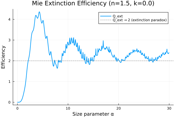
Effect of Absorption on Scattering (Fig. 15.5)
For absorbing particles ($k > 0$), the single-scattering albedo $\omega$ decreases, indicating a larger fraction of extinction is due to absorption.
alpha_range = 0.01:0.05:20.0

# Non-absorbing (water-like)
Q_ext_water = [Aerosol.mie_Q_ext(α, 1.33, 0.0) for α in alpha_range]
Q_scat_water = [Aerosol.mie_Q_scat(α, 1.33, 0.0) for α in alpha_range]
Q_abs_water = Q_ext_water .- Q_scat_water

# Moderately absorbing
Q_ext_mod = [Aerosol.mie_Q_ext(α, 1.5, 0.1) for α in alpha_range]
Q_scat_mod = [Aerosol.mie_Q_scat(α, 1.5, 0.1) for α in alpha_range]
Q_abs_mod = Q_ext_mod .- Q_scat_mod

# Strongly absorbing (carbon-like)
Q_ext_carbon = [Aerosol.mie_Q_ext(α, 1.95, 0.79) for α in alpha_range]
Q_scat_carbon = [Aerosol.mie_Q_scat(α, 1.95, 0.79) for α in alpha_range]
Q_abs_carbon = Q_ext_carbon .- Q_scat_carbon

p1 = plot(alpha_range, Q_ext_water, label = "Q_ext (water)", linewidth = 2)
plot!(alpha_range, Q_ext_mod, label = "Q_ext (n=1.5, k=0.1)", linewidth = 2)
plot!(alpha_range, Q_ext_carbon, label = "Q_ext (carbon)", linewidth = 2)
xlabel!("Size parameter α")
ylabel!("Q_ext")
title!("Extinction Efficiency for Different Materials")

p2 = plot(alpha_range, Q_abs_water, label = "Q_abs (water)", linewidth = 2)
plot!(alpha_range, Q_abs_mod, label = "Q_abs (n=1.5, k=0.1)", linewidth = 2)
plot!(alpha_range, Q_abs_carbon, label = "Q_abs (carbon)", linewidth = 2)
xlabel!("Size parameter α")
ylabel!("Q_abs")
title!("Absorption Efficiency for Different Materials")

plot(p1, p2, layout = (2, 1), size = (700, 600))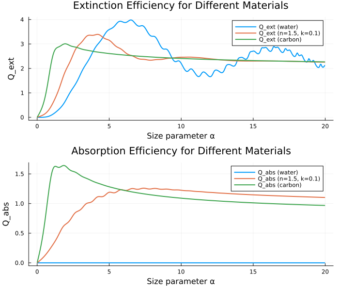
Single-Scattering Albedo vs. Size Parameter
The single-scattering albedo $\omega = Q_{\text{scat}} / Q_{\text{ext}}$ characterizes the relative importance of scattering vs. absorption.
alpha_range = 0.1:0.05:20.0

ω_water = [Aerosol.mie_Q_scat(α, 1.33, 0.0) / Aerosol.mie_Q_ext(α, 1.33, 0.0)
           for α in alpha_range]
ω_mod = [Aerosol.mie_Q_scat(α, 1.5, 0.1) / Aerosol.mie_Q_ext(α, 1.5, 0.1)
         for α in alpha_range]
ω_carbon = [Aerosol.mie_Q_scat(α, 1.95, 0.79) / Aerosol.mie_Q_ext(α, 1.95, 0.79)
            for α in alpha_range]

plot(alpha_range, ω_water, label = "Water (n=1.33, k≈0)", linewidth = 2)
plot!(alpha_range, ω_mod, label = "Moderate absorption (n=1.5, k=0.1)", linewidth = 2)
plot!(alpha_range, ω_carbon, label = "Carbon (n=1.95, k=0.79)", linewidth = 2)
xlabel!("Size parameter α")
ylabel!("Single-scattering albedo ω")
title!("Single-Scattering Albedo (Eq. 15.5)")
ylims!(0, 1.05)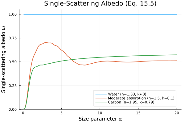
Mass Extinction Efficiency (Fig. 15.7)
The mass extinction efficiency $E_{\text{ext}}$ peaks at particle diameters comparable to the wavelength of light, making submicron particles most efficient at scattering and absorbing radiation per unit mass.
D_p_range = 0.01e-6:0.01e-6:2.5e-6  # 0.01 to 2.5 μm
λ = 550e-9  # 550 nm

# Ammonium sulfate: n=1.521, k≈0, ρ=1770 kg/m³
n_sulfate = 1.521
k_sulfate = 0.0
ρ_sulfate = 1770.0

E_ext_sulfate = Float64[]
for D_p in D_p_range
    α = π * D_p / λ
    Q_ext = Aerosol.mie_Q_ext(α, n_sulfate, k_sulfate)
    push!(E_ext_sulfate, 3 * Q_ext / (2 * ρ_sulfate * D_p))
end

# Carbon: n=1.95, k=0.79, ρ=2000 kg/m³
n_carbon = 1.95
k_carbon = 0.79
ρ_carbon = 2000.0

E_ext_carbon = Float64[]
for D_p in D_p_range
    α = π * D_p / λ
    Q_ext = Aerosol.mie_Q_ext(α, n_carbon, k_carbon)
    push!(E_ext_carbon, 3 * Q_ext / (2 * ρ_carbon * D_p))
end

D_p_um = collect(D_p_range) .* 1e6  # Convert to μm for plotting

plot(D_p_um, E_ext_sulfate, label = "(NH₄)₂SO₄", linewidth = 2)
plot!(D_p_um, E_ext_carbon, label = "Elemental carbon", linewidth = 2)
xlabel!("Particle diameter Dₚ (μm)")
ylabel!("Mass extinction efficiency E_ext (m²/kg)")
title!("Mass Extinction Efficiency at λ=550 nm (Eq. 15.41)")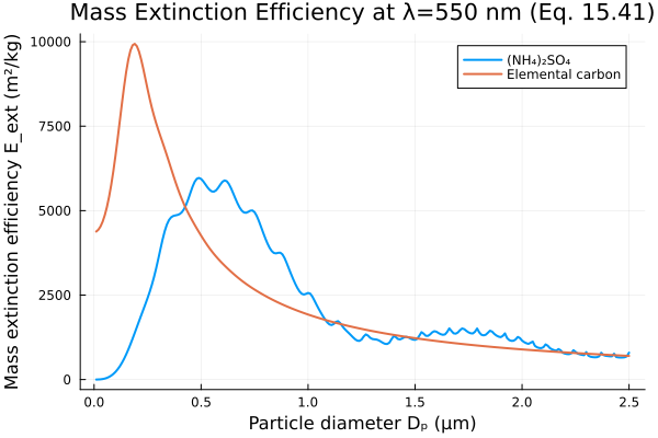
Rayleigh Scattering Regime
In the Rayleigh regime ($\alpha \ll 1$), the full Mie solution reduces to simple closed-form expressions. The key feature is that scattering efficiency scales as $\alpha^4$ (equivalently $1/\lambda^4$), explaining why the sky is blue.
alpha_range_small = 0.001:0.001:0.1

Q_scat_mie = [Aerosol.mie_Q_scat(α, 1.5, 0.0) for α in alpha_range_small]
Q_scat_rayleigh = [(8/3) * α^4 * ((1.5^2 - 1)/(1.5^2 + 2))^2 for α in alpha_range_small]

plot(alpha_range_small, Q_scat_mie, label = "Mie (full)", linewidth = 2)
plot!(alpha_range_small, Q_scat_rayleigh,
    label = "Rayleigh (Eq. 15.19)", linewidth = 2, linestyle = :dash)
xlabel!("Size parameter α")
ylabel!("Q_scat")
title!("Rayleigh vs. Mie Scattering (n=1.5, k=0)")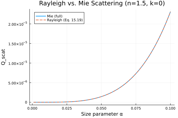
Rayleigh Scattering Coefficient (Problem 15.1A)
The Rayleigh scattering coefficient for air molecules represents the irreducible minimum of light scattering along an atmospheric sight path. At sea level and λ = 550 nm, $b_{sg} \approx 13.2 \times 10^{-6} \text{ m}^{-1}$. The coefficient varies with temperature and pressure according to (Problem 15.1A):
\[b_{sg} = 11.4 \left(\frac{293}{T}\right) p \times 10^{-6} \text{ m}^{-1} \quad (\lambda = 550 \text{ nm})\]
where $T$ is temperature in K and $p$ is pressure in atmospheres.
The Rayleigh scattering coefficient also varies with altitude (page 705):
| Altitude (km) | $b_{sg}$ (10⁻⁶ m⁻¹) |
|---|---|
| 0 | 13.2 |
| 1.0 | 11.4 |
| 2.0 | 10.6 |
| 3.0 | 9.7 |
| 4.0 | 8.8 |
# Rayleigh scattering coefficient at different altitudes
altitudes = [0.0, 1.0, 2.0, 3.0, 4.0]  # km
b_sg_values = [13.2, 11.4, 10.6, 9.7, 8.8] .* 1e-6  # m^-1

bar(altitudes, b_sg_values .* 1e6, label = "b_sg",
    xlabel = "Altitude (km)", ylabel = "b_sg (10⁻⁶ m⁻¹)",
    title = "Rayleigh Scattering Coefficient vs Altitude (λ=520nm)")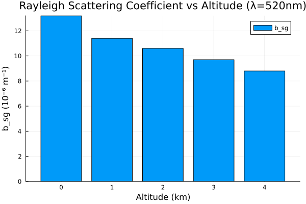
Visibility and Extinction
The Koschmeider equation (Eq. 15.36) relates visual range to extinction coefficient. At sea level in a clean Rayleigh atmosphere ($b_{\text{ext}} \approx 13.2 \times 10^{-6} \text{ m}^{-1}$), the maximum visual range is approximately 296 km.
b_ext_range = 1e-5:1e-5:1e-3  # Extinction coefficient range (m^-1)
x_v = 3.912 ./ b_ext_range  # Koschmeider equation

plot(b_ext_range .* 1e6, x_v ./ 1000, label = "Visual range",
    linewidth = 2, xscale = :log10)
xlabel!("Extinction coefficient b_ext (10⁻⁶ m⁻¹)")
ylabel!("Visual range xᵥ (km)")
title!("Koschmeider Equation (Eq. 15.36)")